
Introduction
As usual, pull the files from the skeleton and make a new IntelliJ project.
Over the past few labs, we have analyzed the performance of algorithms for access and insertion into binary search trees under the assumption that the trees were balanced. Informally, that means that the paths from root to leaves are all roughly the same length, resulting in a runtime logarithmic to the number of items. Otherwise, we would have to worry about lopsided, unbalanced trees in which search is linear rather than logarithmic.
Unfortunately, this balancing doesn’t happen automatically, and we have seen how to insert items into a binary search tree to produce worst-case search behavior. In this lab we will be exploring different techniques which will actually allow us to claim that the height of the tree is indeed logarithmic to the number of items contained in the tree. There are two approaches we can take to make tree balancing happen:
- Incremental balancing
- At each insertion or deletion we do a bit of work to keep the tree balance
- All-at-once balancing
- We don’t do anything to keep the tree balanced until it gets too lopsided, then we completely rebalance the tree.
In the activities of this segment, we will start by analyzing some tree balancing code. Then, we will explore how much work is involved in maintaining complete balance. Finally, we’ll move on to explore three kinds of balanced search trees: B-trees, red-black trees, and left-leaning red-black trees.
Exercise: sortedIterToTree
Implementation
In BST.java, complete the sortedIterToTree method which should build a balanced binary search tree out of an Iterator that returns the items in sorted order.
Warning: This problem is challenging. Don’t spend too much time on it and come back to it at the end of the lab. Talk to your lab partner and let the ideas mingle in the back of your mind as you work through the rest of lab.
Hint: Recursion! Think about the parameters and the order of recursive calls. The very first item in the iterator is also the first item in the inorder traversal of the tree and, therefore, the leftmost child of the balanced binary search tree.
Draw out a couple of cases by hand and break down what needs to be done. There is only one
Iteratorobject (it will be passed through recursive calls), so make sure you think about the order things are being returned from theIteratorand how to construct a tree from it!
You may notice that in our BST, the items are of type Object. However, in previous labs we have seen that the items must be Comparable. Why is this the case? It’s because you shouldn’t need to ever do any comparisons yourself. Just trust that the order of the items returned from the Iterator is correct.
Runtime
Spend some time to discuss what the runtime is for sortedIterToTree, where \(N\) is the length of the iterator. Do you think there is a faster way to do? What is the fastest runtime you think it could be done in? Discuss with your partner, and ask an academic intern or your TA if you want to discuss more!
2-3-4 Trees
The first balanced search tree we’ll examine is the 2-3-4 tree. 2-3-4 trees guarantee \(O(\log N)\) height in any case. That is, the tree is always balanced by height.
2-3-4 trees are named that way because each non-leaf node can have either 2, 3, or 4 children. Additionally, any non-leaf node must have one more child than it does keys. That means that a node with 1 key must have 2 children, 2 keys with 3 children, and 3 keys with 4 children.
Here’s an example of a 2-3-4 tree:
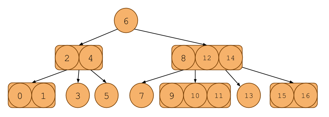
Notice that it looks like a binary search tree, except each node can contain 1, 2, or 3 items rather than just 1. In addition, the tree also follows the ordering invariants of the binary search tree. For example, take the [2, 4] node. Each key in the subtree rooted at the first child has items less than 2. Each key in the second subtree has items between 2 and 4. Each key in the third subtree has items greater than 4. This extends to nodes with more or less keys as well. We can take advantage of this to construct a search algorithm similar to the search algorithm for binary search trees.
Discussion: 2-3-4 Tree Height
What does the invariant that a 2-3-4 tree has one more child than keys tell you about the length of the paths from the root to leaf nodes? How does that keep the 2-3-4 tree balanced? Discuss this with your partner.
Insertion into a 2-3-4 Tree
Although searching in a 2-3-4 tree is like searching in a BST, inserting a new item is a little different.
Like a BST, we always insert the new key at a leaf node. We must find the correct place for the key that we insert to go by traversing down the tree, and then insert the new key into the appropriate place in the existing leaf. However, unlike in a BST, nodes themselves in a 2-3-4 tree can be modified as a result of insertion if a leaf node is able to accept more keys.
Suppose we have the following 2-3-4 tree:
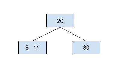
If we were to insert 10 into the tree, we first traverse down the tree until we find the proper leaf node to insert it into. We subsequently find the leaf node that contains 8 and 11. That node still has room (because a node can contain up to 3 keys), and we can insert 10 between 8 and 11, leaving us with a three key node, as shown below.
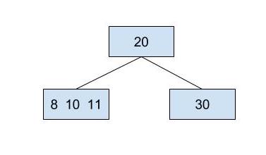
However, what if the leaf node we choose to insert into already has 3 keys? Even though we’d like to put the new item there, it won’t fit because nodes can have no more than 3 keys. What should we do?
The solution is to push up the middle key in the node to the parent, which will split up the node into two single nodes. Then, we will add the key that we are trying to insert into the correct place.
It is possible that this will cause the parent or the parent’s parent to have too many keys. In cases like this, we will repeat this process until our tree has no more nodes with 4 keys in it.
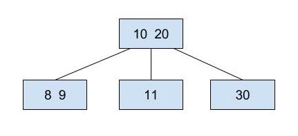
Let’s try to insert 9 into the 2-3-4 tree above.
We must first find which leaf to insert into. 9 is smaller than 20, so we go down to the left. Then we find the leaf that we would like to insert into. Because this node has 3 keys, [8, 10, 11], we push up the middle key (10), then split the 8 and the 11 into separate nodes. We insert 9 into the node with 8 in it, as seen below.
There is one little special case we have to worry about when it comes to inserting, and that’s if the root is a 3-key node. Roots don’t have a parent to push the middle key to. In that case, we still push up the middle key and instead of giving it to the parent, we make it the new root. Only when this happens does the height of the 2-3-4 tree increase.
Exercise: Growing a 2-3-4 Tree
Exercise 1
Insert 5, 7, and 12 into the 2-3-4 tree above. Then, compare your answer with your partner’s.
Exercise 2
Suppose the keys 1, 2, 3, 4, 5, 6, 7, 8, 9, and 10 are inserted sequentially into an initially empty 2-3-4 tree. Which insertion causes the second split to take place?
Try to add these keys to an empty tree, and discuss with your partner your output.
If you want to check your work, consider using this visualization tool from the University of San Francisco. Make sure to set the degree of the tree appropriately. They have a few more interesting visualizations on their site if you want to use as a resource at a later point.
Removal from a 2-3-4 Tree
We will not be covering how to remove from a 2-3-4 tree in this course, but notes on how to do so are in Shewchuk’s notes. The idea behind removal is similar to removal from a BST. Like in insertion, we modify nodes as we find what to delete. Instead of getting rid of 3-key nodes, remove will create 3-key nodes. Again, you will not be responsible on understanding the exact mechanics of the removal algorithm.
B-trees
A 2-3-4 tree is a special case of a structure called a B-tree and its name is sometimes abbreviated as 2-4 tree (captures the minimum and maximum number of children that a node can have rather than all values of children that a node can have). Other types of B-trees include 2-3 trees, 2-3-4-5 trees (often called 2-5 trees), etc. As you can see, what varies among B-trees is the number of keys / subtrees per node.
The USF visualization from above is for B-trees of max degree 3 to 7, which means you can visualize 2-3 trees, 2-4 trees, 2-5, trees, 2-6 trees, and 2-7 trees. If you have not already check the visualization out and see how changing the degree changes what happens when you insert values into the tree. The pattern should be much the same as what we have discussed above for 2-3-4 trees with the main difference being how stuffed we let nodes get before we split them.
B-trees with lots of keys per node (on the order of thousands) are especially useful for organizing storage of disk files, for example, in an operating system or database system. Since retrieval from a hard disk is quite slow compared to computation operations involving main memory, we generally try to process information in large chunks in such a situation, in order to minimize the number of disk accesses. The directory structure of a file system could be organized as a B-tree so that a single disk access would read an entire node of the tree. This would consist of, say, the text of a file or the contents of a directory of files.
If you would like a deeper explanation into 2-3 trees / 2-3-4 trees / B-trees then some of the following resources provide other explanations and some of them are a bit more involved than the brief explanation presented here. Note we will also be covering them in lecture this week, and these resources are just meant for extra review later.
- Josh Hug’s textbook Sections 11.1, 11.2, and 11.3.
- Professor Hilfinger’s balanced search slides (contains more than just a discussion about B-trees).
Red-Black Trees
We saw that 2-3-4 trees are balanced, guaranteeing that a path from the root to any leaf is \(O(\log N)\). However, 2-3-4 trees are notoriously difficult and cumbersome to code, with numerous corner cases for common operations. They are still used, but for our purposes you can imagine that you must represent nodes which contain different numbers of items and have different numbers of children. There turns out to be a related balanced search tree with a one to one correspondence to B-tree which many agree to be slightly simpler to implement.
What’s used in practice is a red-black tree (in fact, it is the tree behind Java’s TreeSet and TreeMap). A red-black tree at its core is just a binary search tree like we saw from yesterdays lab, but there are a few additional invariants related to “coloring” each node red or black. As mentioned above this in fact creates a bijection or mapping between 2-3-4 trees and red-black trees!
The consequence is quite astounding: red-black trees maintain the balance of B-trees while inheriting all normal binary search tree operations (a red-black tree is a binary search tree after all) with additional housekeeping. This self-balancing quality is why Java’s TreeMap and TreeSet are implemented as red-black trees!
2-3-4 Tree ↔ Red-Black Tree
Notice that a 2-3-4 tree can have 1, 2, or 3 elements per node, and 2, 3, or 4 pointers to its children. Consider the following B-tree node:

a, b, c, and d are pointers to its children nodes/subtrees. a will have elements less than 4, b will have elements between 4 and 7, c will have elements between 7 and 10, and d will have elements greater than 10.
Let us transform this into a “section” in red-black tree that represents above node:

For each node in the 2-3-4 tree, we have a group of red-black tree nodes (or colored binary search tree nodes) that correspond to it. Each element in a node of a 2-3-4 tree will correspond to the following in a red-black tree:
- Middle element ↔ a black node that is reachable from parent.
- Left element ↔ a red node on the left of the middle element’s black node.
- Right element ↔ a red node on the right of the middle element’s black node.
As a general rule, any red node in a red-black tree will be in the same node as its parent in a B-tree.
Notice that a, b, c, and d are also “sections” that corresponds to a 2-3-4 tree node. Thus, the subtrees will have black root nodes and other colored nodes that follow the above correspondence.
How about a 2-3-4 node with two elements?

This node can be transformed as:

or

Both are valid.
For 2-3-4 node with only one element, it will translate into a single black node in red-black tree.
Discussion: Correspondence
It may be hard to see at first that the balancedness of 2-3-4 tree still holds on red-black tree, and that a red-black tree is still a binary search tree.
Given a 2-3-4 tree, how can we apply the correspondence rule above to determine the maximum height of the corresponding red-black tree? If each 4-child node in the 2-3-4 tree is equivalent to two red nodes and one black node in a red-black tree, what can we say about the height of the red-black tree?
Then, discuss with your partner about which of the following binary search tree operations we can use on red-black trees without any modification.
- Insertion
- Deletion
- Search (is
kin the tree?) - Range Queries (return all items between
aandb)
Exercise: Constructor
Read the code in RedBlackTree.java and BTree.java.
Then, in RedBlackTree.java, implement buildRedBlackTree which returns the root node of the red-black tree which has a one-to-one mapping to the given 2-3-4 tree. For a 2-3-4 tree node with 2 elements in a node, you must use the “larger” element as the black node to pass the autograder tests. This means that a node with two elements should correspond to a black node with a left red child. For the example above, you must use the second representation of red-black tree where 5 is the red node.
If you’re stuck, refer to the example conversions shown above to help you write this method!
Some further tips for writing this method if you are stuck:
- You should be filling in the three cases which correspond to a 2-node, a 3-node, and a 4-node (these number correspond to the number of children each node in the 2-3-4 tree has). For a 2-node, you should need to make one new
RBTreeNodeobject. For a 3-node, you should need to make two newRBTreeNodeobjects. Finally for a 4-node, you should need to make three newRBTreeNodeobjects. - You should rely on the
getItemAtandgetChildAtmethods from theNodeclass which will return the appropriate items and childrenNodes. - Your code should involve the same number of recursive calls to
buildRedBlackTreeas the number of children in theNodeyou are translating, e.g. two recursive calls for a 2-node, three recursive nodes for a 3-node, and four recursive calls for a 4-node. - For all three cases you should only make one of the
RBTreeNodes be a black node. For the cases where you have more than oneRBTreeNodemake sure that you are returning the black node.
Left-Leaning Red-Black Trees
In the last section, we examined 2-3-4 trees their relationship to red-black trees. Here, we want to extend our discussion a little bit more and examine 2-3 trees and left-leaning red-black trees.
2-3 trees are B-trees, just like 2-3-4 trees. However, they can have up to 2 elements and 3 children, whereas 2-3-4 trees could have one more of each. Naturally, we can come up with a red-black tree counterpart. However, since we can only have nodes with 1 or 2 elements, we can either have a single black node (for a one-element 2-3 node) or a “section” with a black node and a red node (for a two-element 2-3 node). As seen in the previous section, we can either let the red node be a left child or a right child. For these trees, we will choose to always let the red node be the left child of the black node. This leads to the name, “left-leaning” red-black tree. An example of a node containing 5 and 9 is shown below:

The advantages of LLRB tree over the usual red-black tree is the relative ease of implementation. Since there are fewer special cases for each “section” that represents a 2-3 node, the implementation is comparatively simpler when compared to that of a red-black tree which corresponds to a 2-3-4 tree.
We should briefly note that vocabulary that we have been using here might begin to get a bit confusing. In the previous section we were dealing with red-black trees which correspond to 2-3-4 trees, and now we are talking about left-leaning red-black trees which correspond to 2-3 trees.
This becomes more even more confusing when we note that we have forced you to make your red-black tree from above have a certain structure which you should now be able to see makes it left leaning. For our class, we will still reserve the usage of left-leaning red-black tree to refer to the 2-3 tree equivalent.
TLDR: Unless otherwise specified assume that when we say left-leaning red black tree we are referring to the 2-3 tree equivalent and when we say red-black tree we are referring to the more general 2-3-4 tree equivalent. In any instances where this discrepancy is important we will clarify and feel free to ask which we are referring to if you think it matters.
Normal binary search tree insertions and deletions can break the red-black tree invariants, so we need additional operations that can “restore” the red-black tree properties. In LLRB trees, there are two key operations that we use to restore the properties: rotations and color flips.
Rotations
Consider the following tree:

a is a subtree with all elements less than 1, b is a subtree with elements between 1 and 7, and c is a subtree with all elements greater than 7. Now, let’s take a look at another tree:

There are few key things to notice:
- The root of the tree has changed from 7 to 1.
a,b, andcare still correctly placed. That is, their items do not violate the binary search tree invariants.- The height of the tree can change by 1.
Here, we call this transition from the first tree to the second a “right rotation on 7”.
Now, convince yourself that if we start on the second tree and perform a “left rotation on 1”, the resulting tree will be the first tree. The two operations are symmetric, and both maintain the binary search tree property!
Discussion: Rotation by Hand
Let’s say we are given an extremely unbalanced binary search tree:

Write down a series of rotations (i.e. rotate right/left on …) that will make tree balanced and have height of 2.
Hint: Two rotations are sufficient.
The following discussion and exercises will rely heavily on performing rotations, so if you need more help understanding what happens in a rotation we strongly recommend discussing with either your partner, an academic intern or your TA.
Exercise: Rotations
Now we have seen that we can rotate the tree to balance it without violating the binary search tree invariants. Now, we will implement it ourselves!
In RedBlackTree.java, implement rotateRight and rotateLeft. For your implementation, make the new root have the color of the old root, and color the old root red.
Hint: The two operations are symmetric. Should the code significantly differ? If you find yourself stuck, take a look at the examples that are shown above!
Color Flip
Now we consider the color flip operation that is essential to LLRB tree implementation. Given a node, this operation simply flips the color of itself, and the left and right children. However simple it may look now, we will examine its consequences later on.
For now, take a look at the implementation provided in RedBlackTree.java.
Insertion
Finally, we are ready to put the puzzles together and see how insertion works on LLRB trees!
Say we are inserting x.
- If the tree is empty, let
xbe the root with black color. - Otherwise, do the normal binary search tree insertion, and color
xred. Then, restore LLRB tree properties.
But, how do we “restore LLRB tree properties”? Let’s list out all the cases that can occur, and how we will deal with each of them.
Case 1
Let’s assume that our new node x is the only child of a black node. That is:

or

Since we decided to make our tree left leaning, we know that the first tree is the valid form. If we end up with the second tree (x > parent) we can apply rotateLeft on parent to get the first tree.
Case 2
Now, let’s consider the case when our new node x becomes a child of a black node which already has a left child, or a child of a red node. This is like trying to insert x into a 2-3 tree node that already has 2 items and 3 children!
Here, we have to deal with 3 different cases, and we will label them case A, B, C.
- Case 2.A
xends up as the right child of the black node.

Notice that for case 2.A, the resulting section is the same as a 2-3 tree node with one extra element:

To fix it, we “split” the 2-3 node into two halves, “pushing” up the middle element to its parent:

Analogously, for our LLRB section, we can apply flipColor on 5. This results in:

Notice that this exactly models the 2-3 node we desired. 5 is now a red node, which means that is is now part of the “parent 2-3 node section.” Now, if 5 as a new red node becomes a problem, we can recursively deal with it as we are dealing with x now. Also, note that the root of the whole tree should always be black, and it is perfectly fine for the root to have two black children. It is simply a root 2-3 node with single element and two children, each with single element.
- Case 2.B
xends up as the left child of the red node.

In this case, we can apply rotateRight on 5, which will result in:

This should look familiar, since it is exactly case 2.A that we just examined before! After a rotation, our problem reduces to solving case 2.A. Convince yourself that rotation performed here correctly handles the color changes and maintains the binary search tree properties.
- Case 2.C
xends up as the right child of the red node.

In this case, we can apply rotateLeft on 1, which will result in:

This also should look familiar, since it is exactly case 2.B that we just examined. We just need one more rotation and color flip to restore LLRB properties.
Deletion
Deletion deals with many more corner cases and is generally more difficult to implement. For time’s sake, deletion is left out for this lab.
If you would like a deeper explanation into red-black trees then some of the following resources provide other explanations and some of them are a bit more involved than the explanation presented here. Note we will also be covering them in lecture this week, and these resources are just meant for extra review later.
- Josh Hug’s textbook Sections 11.4 and 11.5.
- Josh Hug’s red-black tree lecture videos. (I personally found this lecture really illuminating especially how he compares B-trees to their red-black tree counterparts -Matt)
- Professor Hilfinger’s balanced search slides (contains more than just a discussion about B-trees).
Exercise: insert
Now, we will implement insert in RedBlackTree.java. We have provided you with most of the logic structure, so all you need to do is deal with normal binary search tree insertion and handle case A, B, and C. Make sure you follow the steps from all the cases very carefully! The root of the RedBlackTree should always be black.
Use the helper methods that have already been provided for you in the skeleton files (flipColors and isRed) and your rotateRight and rotateLeft methods to simplify the code writing!
If you’re stuck, write a recursive helper method similar to how we’ve seen insert implemented in previous labs!
- What should the return value be? (Hint: It’s not
void.) - What should the arguments be?
In addition, think about the similarities between cases 2.A, 2.B, and 2.C, and think about how you can integrate those similarities to simplify your code. Feel free to discuss all these points with your lab partner and the lab staff.
Discussion: insert Runtime
We have seen that even though LLRB trees guarantee that the tree will be almost balanced, the LLRB tree insert operation requires many rotations and color flips. Examine the procedure for insert and convince yourself and your partner that insert still takes \(O(\log N)\) as in balanced binary search trees.
Hint: How long is the path from root to the new leaf? For each node along the path, are additional operations limited to some constant number? What does that mean?
Other Balanced Trees
Balanced search is a very important problem in computer science which has garnered many unique and diverse solutions. We have chose two common solutions to the problem to explore in depth. It is also useful to know about other alternatives but we will not expect you to fully understand how they work. Two other interesting solutions to this problem are presented below.
AVL Trees
AVL trees (named after their Russian inventors, Adel’son-Vel’skii and Landis) are height-balanced binary search trees, in which information about tree height is stored in each node along with the item. Restructuring of an AVL tree after insertion is done via a familiar process of rotation, but without color changes.
Splay Trees
Another type of self-balancing BST is called the splay tree. Like other self-balancing trees (AVL, red-black), a splay tree uses rotations to keep itself balanced. However, for a splay tree, the notion of what it means to be balanced is different. A splay tree doesn’t care about differing heights of subtrees, so its shape is less constrained. All a splay tree cares about is that recently accessed nodes are near the top. Upon insertion or access of an item, the tree is adjusted so that item is at the top. Upon deletion, the item is first brought to the top and then deleted.
If you would like to do some more reading about either of these trees, their Wikipedia articles are a great place to start.
Deliverables
- Complete the
sortedIterToTreemethod fromBST.java. - Complete the following methods in
RedBlackTree.java:buildRedBlackTreerotateRightandrotateLeftinsert