bestCount (A) + bestCount (B) + bestCount (C)
A. Intro
Pull the files for lab 7 from the skeleton.
Learning Goals
In this lab, we consider ways of measuring the efficiency of a given code segment. Given a function f, we want to find out how fast that function runs. One way of doing this is to take out a stopwatch and measuring exactly how much time it takes for f to run on some input. However, we'll see later that there are problems with using elapsed time for this purpose.
Instead, we'll use an estimate of how many steps a function f needs to perform to complete execution as a function of its input. We'll first introduce you to a formal model for precisely counting the number of steps it takes for a function to complete execution. Then, we'll introduce you to the "big-Oh" notation for estimating algorithmic complexity. With "big-Oh" notation, we can say, for example, that determining if an unsorted array contains two identical values takes "$O(N^{2})$ comparisons" in the worst case where $N$ is the number of elements in the array.
Finally, we'll learn how to develop better models for analyzing runtime complexity. Oftentimes, the programs we need to analyze are too complex to solve using only basic counting rules so we need some way of organizing information and reducing the complexity of the problem. In this last section, we'll learn how we can break complex algorithms down into smaller pieces that we can then individually analyze.
B. Estimating efficiency by timing it
Algorithms
An algorithm is a step-by-step procedure for solving a problem. An algorithm is an abstract notion that describes an approach for solving a problem. The code we write in this class, our programs, are implementations of algorithms.
For example, consider the problem of sorting a list of numbers. One algorithm we might use to solve this problem is called bubble sort. Bubble sort tells us we can sort a list by repeatedly looping through the list and swapping adjacent items if they are out of order, until the entire sorting is complete.
Another algorithm we might use to solve this problem is called insertion sort. Insertion sort says to sort a list by looping through our list, taking out each item we find, and putting it into a new list in the correct order.
Several websites like VisuAlgo, Sorting.at, Sorting Algorithms, and USF have developed some animations that can help us visualize these sorting algorithms. Spend a little time playing around with these demos to get an understanding of how much time it takes for bubble sort or insertion sort to completely sort a list. We'll revisit sorting in more detail later in this course, but for now, try to get a feeling of how long each algorithm takes to sort a list. How many comparison does each sort need? And how many swaps?
Since each comparison and each swap takes time, we want to know which is the faster algorithm: bubble sort or insertion sort? And how fast can we make our Java programs that implement them? Much of our subsequent work in this course will involve estimating program efficiency and differentiating between fast algorithms and slow algorithms. This set of activities introduces an approach to making these estimates.
Time Estimates
At first glance, it seems that the most reasonable way to estimate the time an algorithm takes is to measure the time directly. Each computer has an internal clock that keeps track of time, usually in the number of fractions of a second that have elapsed since a given base date. The Java method that accesses the clock is System.currentTimeMillis. A Timer class is provided in Timer.java.
Take some time now to find out
- exactly what value
System.currentTimeMillisreturns, and - how to use the
Timerclass to measure the time taken by a given segment of code.
Exercise: Measuring Insertion Sort
The file Sorter.java contains a version of the insertion sort algorithm you worked earlier. Its main method uses a command-line argument to determine how many items to sort. It fills an array of the specified size with randomly generated values, starts a timer, sorts the array, and prints the elapsed time when the sorting is finished. For example, the commands
javac Sorter.java
java Sorter 300
will tell us exactly how long it takes to sort an array of 300 randomly chosen elements.
Copy Sorter.java to your directory, compile it, and then determine the size of the smallest array that needs 1 second (1000 milliseconds) to sort. An answer within 100 elements is fine.
Discussion: Timing Results
How fast is Sorter.java? What's the smallest array size that you and your partner found that takes at least 1 second to sort?
Compare with other people in your lab. Did they come up with the same number as you?
Why are there differences between some students' numbers and other students' numbers? Why is it that the amount of time it takes to sort 25000 elements isn't always the same? What might contribute to these differences?
C. Analyzing the runtime of a program
Counting Steps
We learned that timing a program wasn't very helpful for determining how good an algorithm is. An alternative approach is step counting. The number of times a given step, or instruction, in a program gets executed is independent of the computer on which the program is run and is similar for programs coded in related languages. With step counting, we can now formally and deterministically describe the runtime of programs.
We define a single step as the execution of a single instruction or primitive function call. For example, the + operator which adds two numbers is considered a single step. We can see that 1 + 2 + 3 can be broken down into two steps where the first is 1 + 2 while the second takes that result and adds it to 3. From here, we can combine simple steps into larger and more complex expressions.
(3 + 3 * 8) % 3This expression takes 3 steps to complete: one for multiplication, one for addition, and one for modulus of the result.
From expressions, we can construct statements. An assignment statement, for instance, combines an expression with one more step to assign the result of the expression to a variable. For example, in the code
int a = 4 * 6;
int b = 9 * (a - 24) / (9 - 7);
each assignment statement takes one additional step on top of however many steps it took to compute the right-hand side expressions. In this case, the first assignment to a takes one step to compute 4 * 6 and one more step to assign the result, 24, to the variable a. Try to calculate the number of steps it takes to assign to b.
It takes 5 steps to assign to b:
(a - 24)9 * (a - 24)(9 - 7)9 * (a - 24) / (9 - 7)- Assignment to
b
Here are some basic rules about what we count as taking a single step to compute:
- Assignment and variable declaration statements
- All unary and binary operators
- Conditional
ifstatements - Function calls
returnstatements
One important case to be aware of is that, while calling a function takes a single step to setup, executing the body of the function may require us to do much more than a single step of work.
Counting Conditionals
With a conditional statement like if, the total step count depends on the outcome of the test. For example, the program segment
if (a > b) {
    temp = a;
    a = b;
    b = temp;
}
can take four steps to execute: one for evaluating the conditional expression a > b and three steps for evaluating each line in the body of the condition. But this is only the case if a > b. If the condition is not true, then it only takes one step to check the conditional expression.
That leads us to consider two quantities: the worst case count, or the maximum number of steps a program can execute, and the best case count, or the minimum number of steps a program needs to execute. The worst case count for the program segment above is 4 and the best case count is 1.
Self-test: if ... then ... else Counting
Consider an if ... then ... else of the form
if (A) {
    B;
} else {
    C;
}
where A, B, and C are program segments. (A might be a method call, for instance.) Give an expression for the best-case step count for the if ... then ... else in terms of best-case counts, bestcount (A), bestcount (B), and bestcount (C).
|
|
Incorrect. If we run the program, will both B and C occur?
|
|
minimum (bestCount (A), bestCount (B), bestCount (C))
|
Incorrect. There's no situation where we can run the program and only one of the statements executes.
|
|
bestCount (A) + minimum (bestCount (B), bestCount (C))
|
Correct!
|
|
bestCount (B) + minimum (bestCount (A), bestCount (C))
|
Incorrect. Does statement B necessarily run? Is there any situation where we could skip A?
|
|
bestCount (C) + minimum (bestCount (A), bestCount (B))
|
Incorrect. Does statement C necessarily run? Is there any situation where we could skip A?
|
Self-test: Counting Steps with a Loop
Consider the following program segment.
for (int k = 0; k < N; k++) {
    sum = sum + 1;
}
In terms of $N$, how many operations are executed in this loop? Remember that each of the actions in the for-loop header (the initialization of k, the exit condition, and the increment) count too!
$1 + 5N + 1$
It takes 1 step to execute the initialization, int k = 0. Then, to execute the loop, we have the following sequence of steps:
- Check the loop condition,
k < N - Add 1 to the
sum - Update the value of
sumby assignment - Increment the loop counter,
k - Update
kby assignment
This accounts for the first $1 + 5N$ steps. In the very last iteration of the loop, after we increment k such that k now equals $N$, we spend one more step checking the loop condition again to figure out that we need to finally exit the loop.
A More Complicated Loop
Now consider code for the function remove on an array of values of length elements.
void remove(int pos) {
    for (int k = pos + 1; k < length; k++) {
        values[k-1] = values[k];
    }
    length--;
}
The counts here depend on pos. Each column in the table below shows the total number of steps for computing each value of pos.
| category | pos = 0 | pos = 1 | pos = 2 | ... | pos = length - 1 |
|---|---|---|---|---|---|
| pos + 1 | 1 | 1 | 1 | 1 | |
assignment to k |
1 | 1 | 1 | 1 | |
| loop conditional | length |
length - 1 |
length - 2 |
1 | |
increment to k |
length - 1 |
length - 2 |
length - 3 |
0 | |
update k |
length - 1 |
length - 2 |
length - 3 |
0 | |
| array aaccess | length - 1 |
length - 2 |
length - 3 |
0 | |
| array assignment | length - 1 |
length - 2 |
length - 3 |
0 | |
decrement to length |
1 | 1 | 1 | 1 | |
assignment to length |
1 | 1 | 1 | 1 | |
| Total count | 5 * length |
5 * length - 4 |
5 * length - 8 |
5 |
We can summarize these results as follows: a call to remove with argument pos requires in total:
- 1 step to calculate
pos + 1 - 1 step to make the initial assignment to
k - $\texttt{length} - \texttt{pos}$ loop tests
- $\texttt{length} - \texttt{pos} - 1$ increments of
k - $\texttt{length} - \texttt{pos} - 1$ reassignments to
k - $\texttt{length} - \texttt{pos} - 1$ accesses to
valueselements - $\texttt{length} - \texttt{pos} - 1$ assignments to
valueselements - 1 step to decrement
length - 1 step to reassign to
length
If all these operations take roughly the same amount of time, the total is $5 \times (\texttt{length} - \texttt{pos})$. Notice how we write the number of statements as a function of the input argument. For a small value of pos, the number of steps executed will be greater than if we had a larger value of pos. And vice versa: a larger value of pos will reduce the number of steps we need to execute.
Step Counting in Nested Loops
To count steps in nested loops, you compute inside out. As an example, we'll consider an implementation of the function removeZeroes.
void removeZeroes() {
    int k = 0;
    while (k < length) {
        if (values[k] == 0) {
            remove(k);
        } else {
            k++;
        }
    }
}
Intuitively, the code should be slowest on an input where we need to do the most work, or an array of values full of zeroes. Here, we can tell that there is a worst case—removing everything—and a best case, removing nothing. To calculate the runtime, like before, we start by creating a table to help organize information.
| category | best case | worst case |
|---|---|---|
assignment to k |
1 | 1 |
| loop conditional | length + 1 |
length + 1 |
| array accesses | length |
length |
| comparisons | length |
length |
| calls to remove | 0 | length |
| k + 1 | length |
0 |
update to k |
length |
0 |
In the best case, we never call remove so its runtime is simply the sum of the rows: bestCount (removeZeroes) = $1 + 5 \times \texttt{length} + 1$.
The only thing left to analyze is the worst-case scenario. Remember that the worst case makes length total calls to remove. We already approximated the cost of a call to remove for a given pos and length value earlier: $5 \times (\texttt{length} - \texttt{pos})$.
In our removals, pos is always 0, and only length is changing. The total cost of the removals is shown below.
$$(5 \times \texttt{length}) + (5 \times (\texttt{length} - 1)) + \cdots + (5 \times (0)) \\ = 5 \times ((\texttt{length}) + (\texttt{length} - 1) + \cdots + (0))$$
The challenge now is to simplify the expression. A handy summation formula to remember is
$$1 + 2 + \cdots + k = \frac{k(k + 1)}{2}$$
This lets us simplify the cost of removals. Remembering to factor in the steps in the table, we can now express the worstCount (removeZeroes) as:
$$5 \times \frac{\texttt{length}(\texttt{length})}{2} + 3 \times \texttt{length} + 2$$
That took... a while.
D. Abbreviated Estimates
Estimation with Proportional To
Producing step count figures for even those simple program segments took a lot of work. But normally we don't actually need an exact step count but rather just an estimate of how many steps will be executed.
We can say that a program segment runs in time proportional to a given expression, where that expression is in simplest possible terms. Here, proportional to means within a constant multiple of.
Thus $2N + 3$ is "proportional to $N$" since it's approximately $2 \times N$. Likewise, $3N^{5} + 19N^{4} + 35$ is "proportional to $N^{5}$" since it's approximately $3 \times N^{5}$. As $N$ approaches infinity, the approximation better models the function's real runtime.
Basically, what we're doing here is discarding all but the most significant term of the estimate and also discarding any constant factor of that term. In a later section, we can show exactly why this holds with a more formal notation.
Applying this estimation technique to the removeZeroes method above results in the following estimates:
- The best case running time of
removeZeroesis proportional to the length of the array, or $N$ if $N$ is the length of the array. This is because, in the best case, the true step count, $5 \times \texttt{length} + 2$, is proportional to $\texttt{length}$. - The worst case running time of
removeZeroesis proportional to the square of the length of the array, or $N^{2}$ if $N$ is the length of the array. This is because, in the worst case, the true step count, $5 \times \frac{\texttt{length}(\texttt{length} + 1)}{2} + 3 \times \texttt{length} + 2$, is proportional to $\texttt{length}^{2}$.
Asymptotic Analysis with Big-Theta
A notation often used to provide even more concise estimates is big-Theta, represented by the symbol $\Theta$. Say we have two functions $f(n)$ and $g(n)$ that take in non-negative integers and return real values. We could say
$f(n) \text{ is in } \Theta(g(n))$
if and only if $f(n)$ is proportional to $g(n)$ as $n$ approaches infinity.
Why do we say "in" $\Theta$? You can think of $\Theta(g(n))$ as a set of functions that all grow proportional to $g$. When we claim that $f$ is in this set, we are claiming that $f$ is a function that grows proportional to $g$.
There are analogous notations called big-Oh ($Ο$) and big-Omega ($\Omega$), where big-Oh is used for upper-bounding and big-Omega is used for lower-bounding. If $f(n)$ is in $O(g(n))$, it means $f$ is in a set of functions that are upper-bounded by $g$. Likewise, if $f(n)$ is in $\Omega(g(n))$, it means $f$ is in a set of functions that are lower-bounded by $g$.
Formal Definition of Big-Oh
In this section, we provide a more formal, mathematical definition of big-Oh notation. These are two equivalent definitions of the statement $f(n) \text{ is in } O(g(n))$:
- There exist positive constants M and N such that for all values of $n > N$, $f(n) < M \times g(n)$. Example: Given $f(n) = n^{2}$ and $g(n) = n^{3}$, is $f(n) \text{ in } O(g(n))$? Is $g(n) \text{ in } O(f(n))$? We can choose $M = 1$ and $N = 1$. We know that for all $n > 1$, $n^{2} < 1 \times n^{3}$. Therefore, $f(n) \text{ is in } O(g(n))$. However, it is impossible to find positive integers $M$ and $N$ such that $n^{3} < M \times n^{2}$ for all $n > N$. Notice that to satisfy the inequality $n^{3} < M \times n^{2}$, $n$ must be less than $M$. But since $M$ a constant, $n^{3} < M \times n^{2}$ does not hold for arbitrarily large values of $n$.
$f(n) \in O(g(n)) \Longleftrightarrow \lim\limits_{n \to \infty} \frac{f(n)}{g(n)} < \infty$
This means, essentially, that for very large values of $n$, $f$ is not a lot bigger than $g$.
Example: Given $f(n) = n^{5}$ and $g(n) = 5^{n}$, is $f(n) \text{ in } O(g(n))$? Is $g(n) \text{ in } O(f(n))$?
After repeatedly applying L'hopital's rule, we see that $f(n) \text{ is in } O(g(n))$:
$$\lim\limits_{n \to \infty} \frac{f(n)}{g(n)} = \lim\limits_{n \to \infty} \frac{n^{5}}{5^{n}} = \lim\limits_{n \to \infty} \frac{5n^{4}}{5^{n} \log 5} = \cdots = \lim\limits_{n \to \infty} \frac{5!}{5^{n} \log^5 5} = 0$$
However, $g(n)$ is not in $O(f(n))$:
$$\lim\limits_{n \to \infty} \frac{g(n)}{f(n)} = \lim\limits_{n \to \infty} \frac{5^{n}}{n^{5}} = \lim\limits_{n \to \infty} \frac{5^{n} \log 5}{5n^{4}} = \cdots = \lim\limits_{n \to \infty} \frac{5^{n} \log 5}{5!} = \infty$$
Formal Definitions of big-Omega and big-Theta
There are a few different ways to define big-Omega and big-Theta.
big-Omega:
$$f(n) \in \Omega(g(n)) \Longleftrightarrow g(n) \in O(f(n)) \Longleftrightarrow \lim\limits_{n \to \infty} \frac{f(n)}{g(n)} > 0$$
big-Theta:
$$f(n) \in \Theta(g(n)) \Longleftrightarrow f(n) \in O(g(n)) \text{ AND } g(n) \in O(f(n)) \\ \Longleftrightarrow \lim\limits_{n \to \infty} \frac{f(n)}{g(n)} = c \\ \text{ for some constant } 0 < c < \infty$$
Orders of Growth are Proportional to a Given Variable
You may have observed, in our analysis of remove, that we were careful to make clear what the running time estimate depended on, namely the value of length and the position of the removal.
Unfortunately, students are sometimes careless about specifying the quantity on which an estimate depends. Don't just use $N$ without making clear what $N$ means. This distinction is important especially when we begin to touch on sorting later in the course. It may not always be clear what $N$ means.
Commonly-Occurring Orders of Growth
Here are some commonly-occurring estimates listed from no growth at all to fastest growth.
- constant time
- logarithmic time or proportional to $\log N$
- linear time or proportional to $N$
- quadratic/polynomial time or proportional to $N^{2}$
- exponential time or proportional to $k^{N}$
- factorial time or proportional to $N!$
Logarithmic Algorithms
We will shortly encounter algorithms that run in time proportional to $\log N$ for some suitably defined $N$. Recall from algebra that the base-10 logarithm of a value is the exponent to which 10 must be raised to produce the value. It is usually abbreviated as $\log_{10}$. Thus
- $\log_{10} 1000$ is 3 because $10^{3} = 1000$
- $\log_{10} 90$ is slightly less than 2 because $10^{2} = 100$
- $\log_{10} 1$ is 0 because $10^{0} = 1$
In algorithms, we commonly deal with the base-2 logarithm, written as $\lg$, defined similarly.
- $\lg 1024$ is 10 because $2^{10} = 1024$
- $\lg 9$ is slightly more than 3 because $2^{3} = 8$
- $\lg 1$ is 0 because $2^{0} = 1$
Another way to think of log is the following: $\log_{\text{base}} N$ is the number of times $N$ must be divided by $base$ before it hits 1. For the purposes of determining orders of growth, however, the log base actually doesn't make a difference because, by the change of base formula, we know that any logarithm of $N$ is within a constant factor of any other logarithm of $N$. We usually express a logarithmic algorithm as simply $\log N$ as a result.
Algorithms for which the running time is logarithmic are those where processing discards a large proportion of values in each iterations. The binary search algorithm is an example. We can use binary search in order to guess a number that a person in thinking. In each iteration, the algorithm discards half the possible values for the searched-for number, repeatedly dividing the size of the problem by 2 until there is only one value left.
For example, say you started with a range of 1024 numbers in the number guessing game. Each time you would discard half of the numbers so that each round would have the following numbers under consideration:
| Round # | Numbers left |
|---|---|
| 1 | 1024 |
| 2 | 512 |
| 3 | 256 |
| 4 | 128 |
| 5 | 64 |
| 6 | 32 |
| 7 | 16 |
| 8 | 8 |
| 9 | 4 |
| 10 | 2 |
| 11 | 1 |
We know from above that $\lg 1024 = 10$ which gives us an approximation of how many rounds it will take.
We will see further applications of logarithmic behavior when we work with trees in subsequent activities.
E. Modeling runtime analysis
A Graphical Approach to Analyzing Iteration
We've thus far defined the language of asymptotic analysis and developed some simple methods based on counting the total number of steps. However, the kind of problems we want to solve are often too complex to think of just in terms of number iterations times however much work is done per iteration.
Consider the following function, repeatedSum.
long repeatedSum(int[] values) {
    int N = values.length;
    long sum = 0;
    for (int i = 0; i < N; i++) {
        for (int j = i; j < N; j++) {
            sum += values[j];
        }
    }
    return sum;
}
In repeatedSum, we're given an array of values of length N. We want to take the repeated sum over the array as defined by the following sequence of j's.
$0, 1, 2, 3, \cdots, N - 1$
$1, 2, 3, 4, \cdots, N - 1$
$2, 3, 4, 5, \cdots, N - 1$
Notice that each time, the number of elements, or the iterations of j, being added is reduced by 1. While in the first iteration, we sum over all $N$ elements, in the second iteration, we only sum over $N - 1$ elements. On the next iteration, even fewer: just $N - 2$ elements. This pattern continues until the outer loop, i, has incremented all the way to $N$.
One possible approach to this problem is to draw a bar graph to visualize how much work is being done for each iteration of i. We can represent this by plotting the values of i across the X-axis of the graph and the number of steps for each corresponding value of i across the Y-axis of the graph.
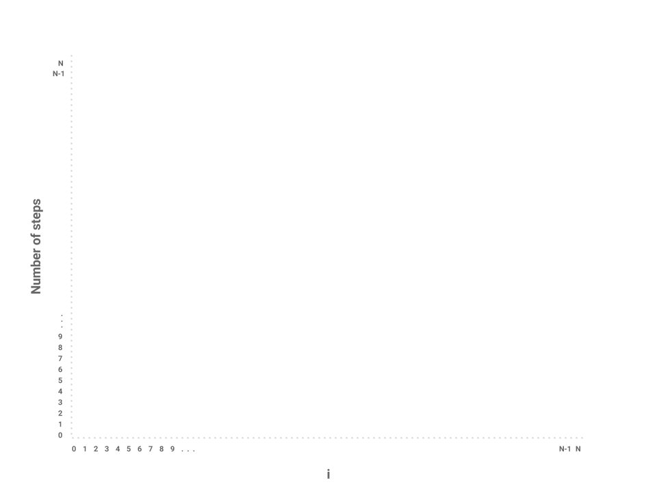
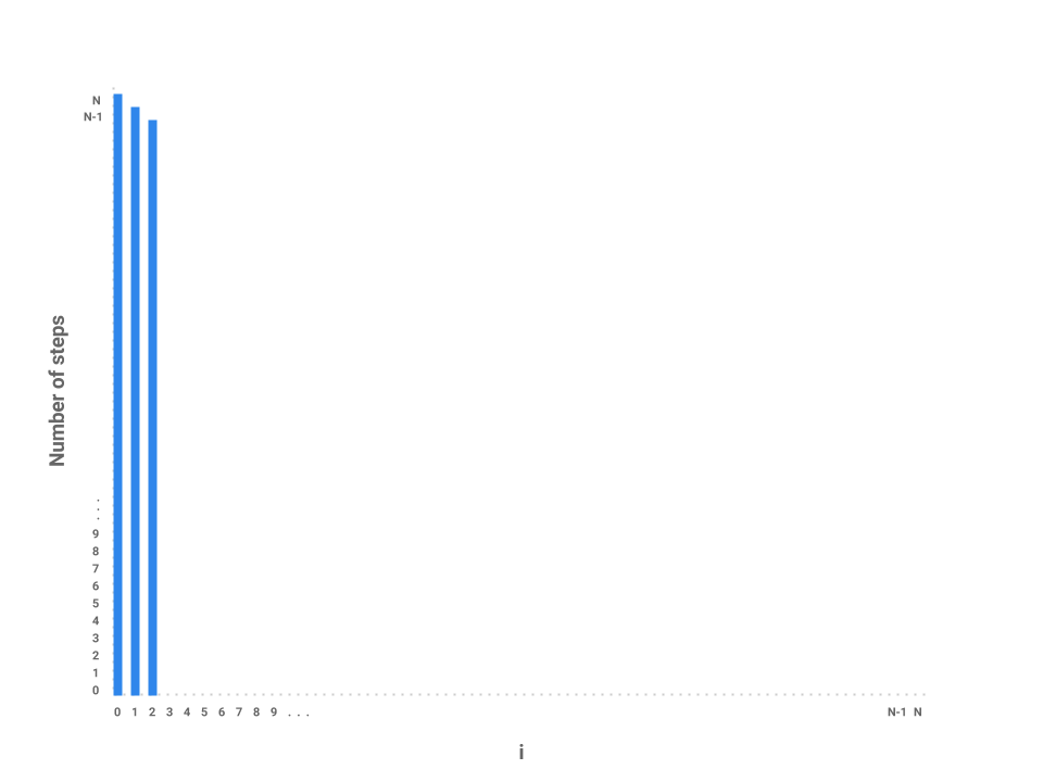
Now, let's plot the amount of work being done on the first iteration of i where i = 0. If we examine this iteration alone, we just need to measure the amount of work done by the j loop. In this case, the j loop does work proportional to $N$ steps as the loop starts at 0, increments by 1, and only terminates when j = N.
How about the next iteration of i? The loop starts at 1 now instead of 0 but still terminates at $N$. In this case, the j loop is proportional to $N - 1$ steps. The next loop, then, is proportional to $N - 2$ steps.
We can start to see a pattern forming. As i increases by 1, the amount of work done on each corresponding j loop decreases by 1. As i approaches $N$, the number of steps in the j loop approaches 0. In the final iteration, i = N-1, the j loop performs work proportional to 1 step.
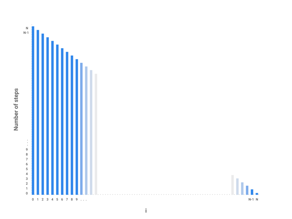
We've now roughly measured each loop proportional to some number of steps. Each independent bar represents the amount of work any one iteration of i will perform. The runtime of the entire function repeatedSum then is the sum of all the bars, or simply the area underneath the line.
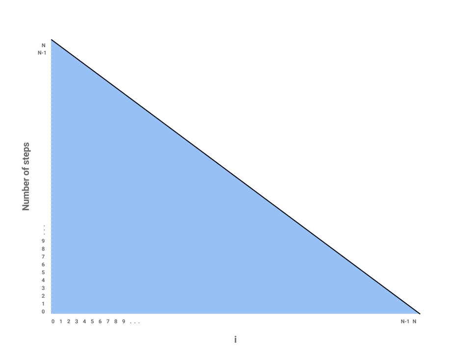
The problem is now reduced to finding the area of a triangle with a base of $N$ and height of also $N$. Thus, the runtime of repeatedSum is in $\Theta(N^{2})$.
We can verify this result mathematically by noticing that the sequence can be described by the following summation:
$1 + 2 + 3 + ... + N = \frac{N(N + 1)}{2}$ or, roughly, $\frac{N^{2}}{2}$ which is in $\Theta(N^{2})$. It's useful to know both the formula as well as its derivation through the graph above.
Tree Recursion
Now that we've learned how to use a bar graph to represent the runtime of an iterative function, let's try the technique out on a recursive function, mitosis.
int mitosis(int N) {
    if (N == 1) {
        return 1;
    }
    return mitosis(N / 2) + mitosis(N / 2);
}
Let's start by trying to map each $N$ over the x-axis like we did before and try to see how much work is done for each call to the function. The conditional contributes a constant amount of work to each call. But notice that in our return statement, we make two recursive calls to mitosis. How do we represent the runtime for these calls? We know that each call to mitosis does a constant amount of work evaluating the conditional base case but it's much more difficult to model exactly how much work each recursive call will do. While a bar graph is a very useful way of representing the runtime of iterative functions, it's not always the right tool for recursive functions.
Instead, let's try another strategy: drawing call trees. Like the graphical approach we used for iteration earlier, the call tree will reduce the complexity of the problem and allow us to find the overall runtime of the program on large values of $N$ by taking the tree recursion out of the problem. Consider the call tree for fib below.
int fib(int N) {
    if (N <= 1) {
        return 1;
    }
    return fib(n - 1) + fib(n - 2);
}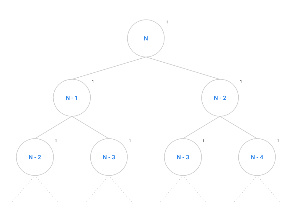
At the root of the tree, we make our first call to fib(n). The recursive calls to fib(n - 1) and fib(n - 2) are modeled as the two children of the root node. We say that this tree has a branching factor of two as each node contains two children. It takes a constant number of instructions to evaluate the conditional, addition operator, and the return statement as denoted by the 1.
We can see this pattern occurs for all nodes in the tree: each node performs the same constant number of operations if we don't consider recursive calls. If we can come up with a scheme to count all the nodes, then we can simply multiply by the constant number of operations to find the overall runtime of fib.
Remember that the number of nodes in a tree is calculated as the branching factor, $k$, raised to the height of the tree, $h$, or $k^{h}$. Spend a little time thinking about the maximum height of this tree: when does the base case tell us the tree recursion will stop?
Self-test: Choosing the Right Notation
Identify the asymptotic runtime complexity of fib(N).
|
$\Theta(N^{2})$
|
Incorrect. Each instance of
fib
makes two recursive calls to
fib
again. This continues for N levels.
|
|
|
$O(N^{2})$
|
Incorrect. Each instance of
fib
makes two recursive calls to
fib
again. This continues for N levels.
|
|
|
$\Theta(2^{N})$
|
Incorrect. The intuition is right, but it's important to notice that, while each call to
fib
makes two more recursive calls to
fib
, the recursive calls are
not
equal as one calls
fib(N - 1)
while the other calls
fib(N - 2)
. The left side of the tree will do significantly more work than the right side of the tree to the point where the runtime is no longer exactly within $\Theta(2^{N})$.
|
|
|
$O(2^{N})$
|
Correct! There's a small but significant difference between big-Oh and big-Theta in this problem as the runtime for
fib
is not exactly $\Theta(2^{N})$ as given by the tight bound, theta. The call tree is actually imbalanced as the left edge contains $N$ nodes but the right edge contains only $N/2$ nodes. We describe this runtime more exactly as $\Theta(1.618^{N})$ which is within $O(2^{N})$ but
not
within $\Theta(2^{N})$.
|
Now, back to mitosis. The problem is setup just like fib except instead of decrementing $N$ by 1 or 2, we now divide $N$ in half each time. Each node performs a constant amount of work but also makes two recursive calls to mitosis(N / 2).
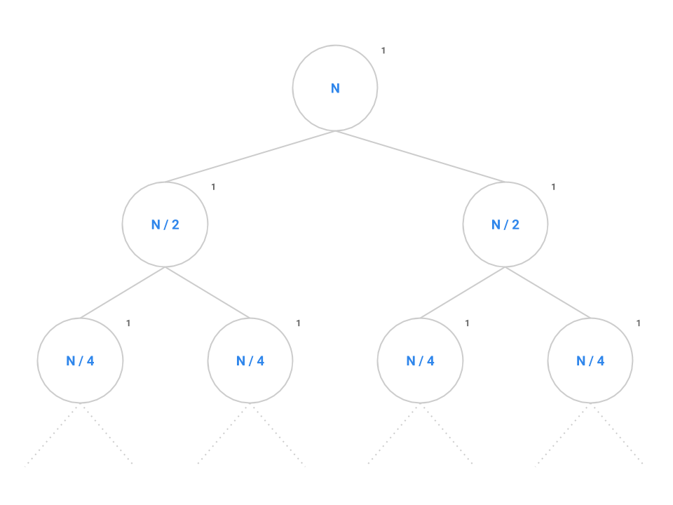
Like before, we want to identify both the branching factor and the height of the tree. In this case, the branching factor is 2 like before. Recall that the series $N, N/2, \cdots , 4, 2, 1$ contains $\log_{2} N$ elements since, if we start at $N$ and break the problem down in half each time, it will take us approximately $\log_{2} N$ steps to completely reduce down to 1.
Plugging into the formula, we get $2^{\log_{2} N}$ nodes which simplifies to $N$. Therefore, $N$ nodes performing a constant amount of work each will give us an overall runtime in $\Theta(N)$.
In general, for a recursion tree, we can think of the total work as $\sum_{\text{layers}} \frac{\text{nodes}}{\text{layer} }\frac{\text{work}}{\text{node}}$ For mitosis, we have $\lg N$ layers, $2^i$ nodes in layer $i$, with $1$ work per node. Thus we see the sumation $\sum_{i = 0}^{\lg N} 2^i (1)$, which is exactly the quantity we just calculated.
F. Practice
Exercise: Complete RuntimeQuiz.java
Look in RuntimeQuiz.java, where we have provided one example and some more common method types for you to analyze the run-time of in asymptotic notation. Fill out the missing fields to correctly match the runtime to the method.
Asymptotic analysis is the primary overarching way we look at efficiency, determining how fast a method is, before we look at the constant factors in a method. Throughout the rest of the class, you should expect to see analysis of each data structure's runtime in asymptotic notation.
Exercise: Analyze DLList
Examine your data structure, the DLList, from the previous lab. In RuntimeQuiz.java, fill out the runtimes in asymptotic notation as you did for the methods, but for your list.
G. Conclusion
Summary
In this section, we learned about three different techniques for analyzing the runtime of program.
- First, we tried to estimate the runtime efficiency of a program by timing it. But we found that the results weren't always the same between different computers or even running at different times.
- Second, we developed the method of counting steps as a deterministic way of calculating the algorithmic complexity of a program. This works well, but it can be challenging to get the exact instruction count. Oftentimes, we don't need exact constants or lower-order terms since, in the long-run, the size of the input, $N$, is the most significant factor in the runtime of a program.
Third, we learned how to estimate the efficiency of an algorithm using proportionality and orders of growth.
- big-Oh describes an upper bound for an algorithm's runtime.
- big-Omega describes a lower bound for an algorithm's runtime.
- big-Theta describes a tight bound for an algorithm's runtime.
In the final section, we applied what we learned about counting steps, estimation, and orders of growth to model algorithmic analysis for larger problems. Two techniques, graphs and call trees, helped us break down challenging problems into smaller pieces that we could analyze individually.
Practical Tips
- Before attempting to calculate a function's runtime, first try to understand what the function does.
- Try some small sample inputs to get a better intuition of what the function's runtime is like. What is the function doing with the input? How does the runtime change as the input size increases? Can you spot any 'gotchas' in the code that might invalidate our findings for larger inputs?
- Try to lower bound and upper bound the function runtime given what you know about how the function works. This is a good sanity check for your later observations.
- If the function is recursive, draw a call tree to map out the recursive calls. This breaks the problem down into smaller parts that we can analyze individually. Once each part of the tree has been analyzed, we can then reassemble all the parts to determine the overall runtime of the function.
- If the function has a complicated loop, draw a bar graph to map out how much work the body of the loop executes for each iteration.
Useful Formulas
- $1 + 2 + 3 + 4 + \cdots + N \text{ is in } \Theta(N^{2})$
- There are $N$ terms in the sequence $1, 2, 3, 4, \cdots, N$
- $1 + 2 + 4 + 8 + \cdots + N \text{ is in } \Theta(N)$
- There are $\lg N$ terms in the sequence $1, 2, 4, 8, \cdots, N$
- The number of nodes in a tree, $N$, is equal to $k^{h}$ where $k$ is the branching factor and $h$ is the height of the tree
- All logarithms are proportional to each other by the Change of Base formula so we can express them generally as just $\log$.
It's worth spending a little time proving each of these to yourself with a visual model!
Deliverables
A quick recap of what you need to do to finish today's lab:
- Look through the Timer class and try timing the algorithm in Sorter.java for different inputs. Discuss with your neighbors what you and your partner came up with.
- Try the self tests on counting instructions.
- Read through the content on asymptotic analysis (big-theta, O, and omega) focusing on how to handle logarithmic, iterative, and recursive algorithms.
- Work through the self-tests on asymptotics.
- Complete the exercises in RunTimeQuiz.java and make sure they pass the autograder tests.