A. Intro

Learning Goals

Pull the skeleton code for lab22 from GitHub.

Today's activities tie up some loose ends in the coverage of sorting. First, an algorithm, derived from Quicksort, to find the kth largest element in an array is presented. We will then look at analyzing the runtime for various sorting algorithms (as well as a bound for runtimes for all comparison-based sorts). Next, the property of stable sorting is discussed. Finally, some linear-time sorting algorithms are described.

B. Quickselect

Finding the Kth Largest Element

Suppose we want to find the kth largest element in an array. We could just sort the array largest-to-smallest and then index into the kth position to do this. Is there a faster way? Finding the kth item ought to be easier since it asks for less information than sorting. Indeed, finding the smallest or largest requires just one pass through the collection.

You may recall the activity of finding the kth largest item (1-based) in a binary search tree. To accomplish this, we augment each node with information about the size of its subtree. The desired item was found as follows:

1. If the right subtree has k-1 items, then the root is the kth item, so return it.
2. If the right subtree has k or more items, find the kth largest item in the right subtree.
3. Otherwise, let j be the number of items in the right subtree, and find the k-j-1th item in the left subtree.

A binary search tree is similar to the recursion tree produced by the Quicksort algorithm. The root of the BST corresponds to the pivot in Quicksort; a lopsided BST, which causes poor search performance, corresponds exactly to a Quicksort in which the divider splits the elements unevenly. We use this similarity to adapt the Quicksort algorithm to the problem of finding the kth largest element.

Here was the Quicksort algorithm.

1. If the collection to be sorted is empty or contains only one element, it's already sorted, so return.
2. Split the collection in two by partitioning around a "divider" element. One collection consists of elements greater than the divider, the other of elements less than or equal to the divider.
3. Quicksort the two subcollections.
4. Concatenate the divider with the sorted large values, and then with the sorted small values.

Discussion: Quickselect

Can you see how you can adapt the basic idea behind the Quicksort algorithm to finding the kth largest element? (Think about how it works in a binary tree!) Describe the algorithm below.

Note: The algorithm's average case runtime will be proportional to N, where N is the total number of items, though it may not be immediately obvious why this is the case.

C. Average Case Runtimes

In previous labs, we looked at amortized analysis, which was a rigorous way to prove an "average" case running time. This was motivated that by the fact that even though the worst case runtime for a single operation could be slow, by looking over a sequence of operations, we can see the runtime could end up being fast.

We will look at another way to prove "average" case running time, through randomized analysis. In sorting algorithms that we covered, such as insertion sort and Quicksort, the runtime depends on random choices. We will use the notion of expectation from probability theory to reason about the random factors in these algorithms and show that the probability of the algorithm running asymptotically slower is low (or high).

Note that there's two different ways of defining average here. In amortized analysis, we care about the average over a series of operations. In randomized analysis, we define the average as what we expect our random factors to look like (which could be the input array or the pivot choice).

Insertion Sort

Let's consider first the case of insertion sort, and define the idea of an inversion. An inversion is a pair of elements $j < k$ such that $j$ comes after k in the input array. That is, $j$ and $k$ are out of order.

This means that the maximum number of inversion in an array is bounded by the number of pairs, and is $\frac{n(n-1)}{2}$.

For every inversion, insertion sort needs to make one swap. Convince yourself that this is true with an example: in the array [1, 3, 4, 2], there are two inversions, (3, 2) and (4, 2), and the key 2 needs to be swapped backwards twice to be in place. Thus the runtime of insertion sort is $\Theta(n + k)$, where k is the number of inversions. Hence, if k is small, linear, or even linearithmic, insertion sort runs quickly (just as fast as, or even faster than, mergesort and Quicksort).

How many inversions are in an average array? Every pair of numbers has an equal chance of being either inverted, or not inverted, so the number of inversions is uniformly distributed between 0 and $\frac{n(n-1)}{2}$; thus the expected (average) number of inversions is precisely the middle, $\frac{n(n-1)}{4}$. This value is in $\Theta(n^2)$, and insertion sort's average case runtime is $\Theta(n^2)$.

Quicksort

The average case runtime of Quicksort depends on the pivot chosen. Recall that in the best case, the pivot chosen is the median, meaning 50% of the elements are on either side of the pivot after partitioning.

The worst possible pivot is the smallest or largest element of the array, meaning 0% or 100% of the elements are on either side of the pivot after partitioning.

Assuming the choice of pivot is uniformly random, the split obtained is uniform random between 50/50 and 0/100. That means in the average case, we expect a split of 25/75. This gives a recursion tree of height $\log_{\frac{4}{3}}(n)$ where each level does $n$ work. Then Quicksort still takes $O(N \log N)$ time in the average case.

How often does the bad-pivot case come up if we pick pivots uniformly at random? Half the array can be considered a bad pivot. As the array gets longer, the probability of picking a bad pivot for every recurisive call to quicksort exponentially decreases.

For an array of length 30, the probability of picking all bad pivots, $\frac{1}{2}^{30} ~= 9.3e-10$, which is approximately the same as winning the powerball: $3.3e-9$.

For an array of length 100, the probability of picking all bad pivots, $7.8e-31$, is so low that if we ran Quicksort every second for 100 billion years, we'd still have a significantly better chance trying to win the lottery in one ticket.

Of course, there's the chance you pick something in between, and the analysis can get far more complicated, especially with variants of Quicksort. For practical purposes, we can treat Quicksort like it's in $O(n \lg n)$.

D. Comparison-sorting Lower Bounds

You may be wondering if it's possible to do better than $O(n \lg n)$ in the worst case for these comparison-based sorts. Read the "A LOWER BOUND ON COMPARISON-BASED SORTING" part from Jonathan Shewchuk's notes on Sorting and Selection. Note that this is mandatory reading and considered a part of the lab.

E. A Linear Time Sort

We just showed that in the worst case, a comparison-based sort (with 2-way decisions) must take at least $\Omega(n \lg n)$ time. (If you didn't catch that, go back and read the notes!!!) But what if instead of making a 2-way true / false decision, we make a k-way decision?

Counting Sort

Suppose you have an array of a million Strings, but you happen to know that there are only three different varieties of Strings in it: "Cat", "Dog", and "Person". You want to sort this array to put all the cats first, then all the dogs, then the people. How would you do it? You could use merge sort or Quicksort and get a runtime proportional to N log N, where N is ~one million. Can you do better?

We think you can. Take a step back and don't think too hard about it. What's the simplest thing you could do?

We propose an algorithm called counting sort. For the above example, it works like this:

1. First create an int array of size three. Call it the counts array. It will count the total number of each type of String.
2. Iterate through your array of animals. Every time you find a cat, increment counts[0] by 1. Every time you find a dog, increment counts[1] by 1. Every time you find a person, increment counts[2] by 1. As an example, the result could be this: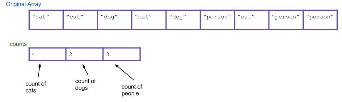
3. Next, create a new array that will be your sorted array. Call it sorted.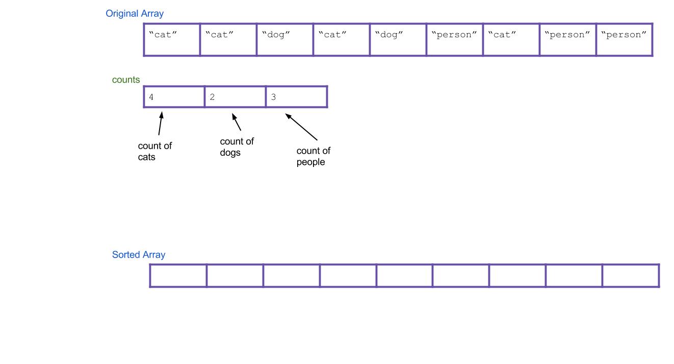
4. Think about it: based on your counts array, can you tell where the first dog would go in the new array? The first person? Create a new array, called starts, that holds this information. We can get this by scanning through the counts array and finding the total number of items to the left of index i. For our example, the result is: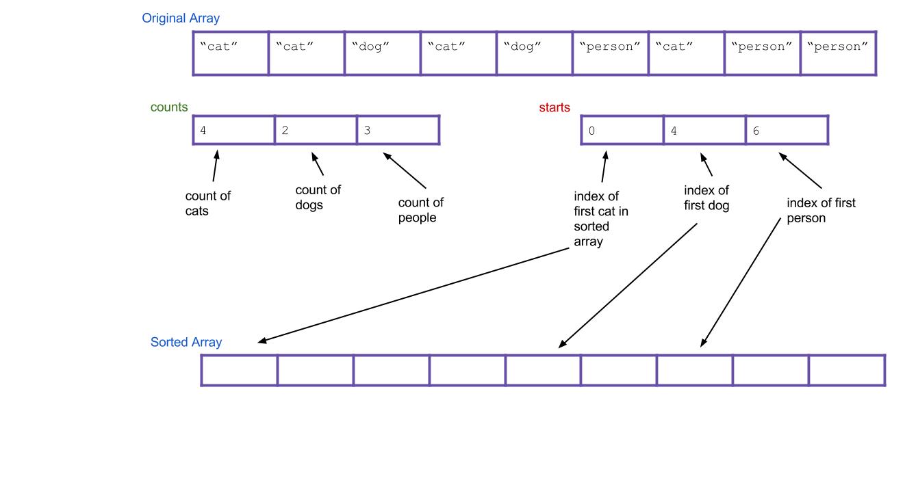
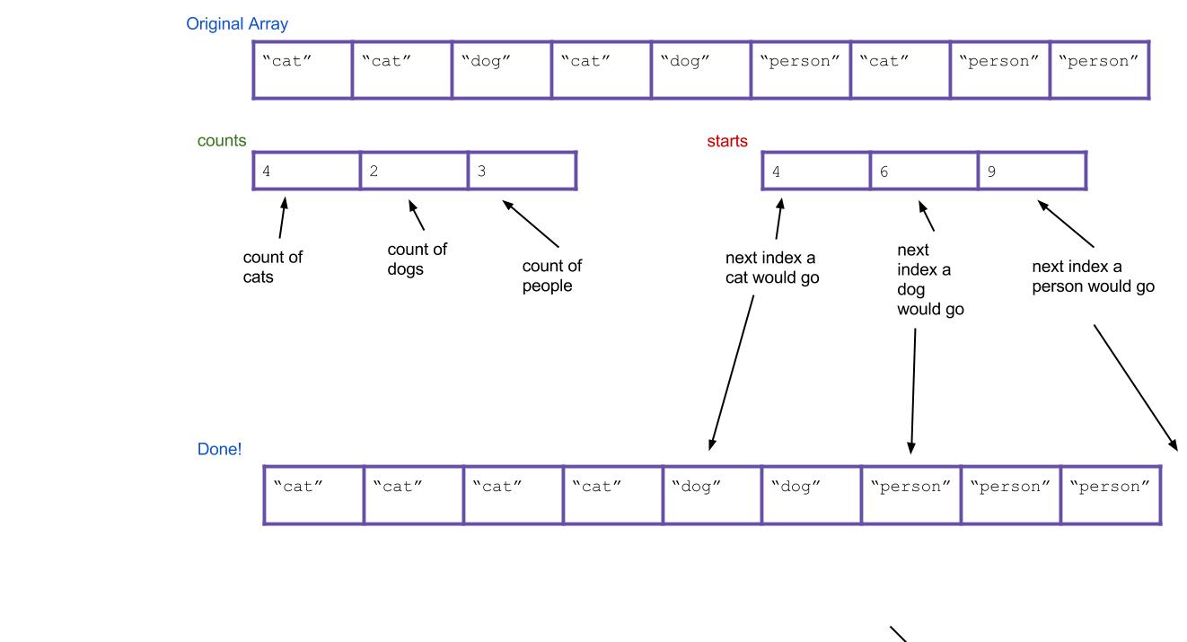
5. Now iterate through all of your Strings, and put them into the right spot. When I find the first cat, it goes in sorted[starts[0]]. When I find the first dog, it goes in sorted[starts[1]]. What about when I find the second dog? It goes in sorted[starts[1]+1], of course. Or, an alternative: I can just increment starts[1] every time I put a dog. Then the next dog will always go in sorted[starts[1]].

Here's what everything would look like after completing the algorithm. Notice that the values of starts have been incremented along the way.

Does the written explanation of counting sort seem complicated? Here is a pretty cool animated version of it that might make it more intuitive.

Exercise: Code Counting Sort

Implement the countingSort method in DistributionSorts.java. Assume the only integers it will receive are 0, 1, 2, 3, 4, 5, 6, 7, 8, and 9.

The Runtime of Counting Sort

Inspect the counting sort method you just wrote. What is its runtime? Consider the following two variables: N: the number of items in the array, and K, the variety of possible items (in the code you wrote, K is the constant 10, but treat it as a variable for this question).

Wow, look at that runtime! Does this mean counting sort is a strict improvement to Quicksort? Nope! Counting sort has two major weaknesses:

• It can only be used to sort discrete values.
• It will fail if K is too large, because creating the intermediate counts array (of size K) will be too slow.

The latter point turns out to be a fatal weakness for counting sort. The range of all possible integers in Java is just too large for counting sort to be practical in general circumstances.

Suddenly, counting sort seems completely useless. Forget about it for now! The next portion of the lab will talk about something completely different. But counting sort will reappear once again when you least expect it...

F. Stability

Stable Sorting

A sorting method is referred to as stable if it maintains the relative order of entries with equal keys. Consider, for example, the following set of file entries:

data.txt    10003   Sept 7, 2005
hw2.java     1596   Sept 5, 2005
hw2.class    4100   Sept 5, 2005

Suppose these entries were to be sorted by date. The entries for hw2.java and hw2.class have the same date; a stable sorting method would keep hw2.java before hw2.class in the resulting ordering, while an unstable sorting method might switch them.

A stable sort will always keep the equivalent elements in the original order, even if you sort it multiple times.

Discussion: Importance of Stability

We described one reason why stability was important: it could help us with the multiple-key sorting example shown above. Can you think of another reason why stability might be important? Describe an application where it matters if the sorting method used is stable.

Optional Exercise: Instability of Selection Sort

In UnstableSelectionSort.java you'll find -- surprise -- an unstable version of selection sort. Verify this fact, and change the method to make the sort stable.

This exercise is now optional!

Quicksort: A Sad Story

Quicksort in its fastest form on arrays is not stable (This version uses two pointers that slide towards each other, using Hoare's partitioning scheme). Aside from its worst case runtime (which in all practical cases, is not relevant/probable), this is Quicksort's major weakness, and the reason why some version of merge sort is often preferred when stability is needed. Of the common implementations of major sorting algorithms (insertion, merge, and quick), only Quicksort's optimized version is not stable.

(The Quicksort you implemented on a linked list is stable, though! Note that this is not the fastest implementation.)

There is a case when stability is not important, however - when sorting primitives, stability of sorts loses its meaning, because there is no value associated with each key. This is the major reason why Arrays.sort uses Dual-Pivot Quicksort in place of the standard Quicksort algorithm and Collections.sort uses a variant of mergesort.

G. Radix Sort

Linear Time Sorting with Distribution Sorts

Aside from counting sort, all the sorting methods we've seen so far are comparison-based, that is, they use comparisons to determine whether two elements are out of order. We also saw the proof that any comparison-based sort needs at least $\Omega(N log N)$ comparisons to sort N elements in the worst case. However, there are sorting methods that don't depend on comparisons that allow sorting of N elements in time proportional to N. Counting sort was one, but turned out to be impractical.

However, we now have all the ingredients necessary to describe radix sort, another linear-time non-comparison sort that can be practical.

Radix Sort

The radix of a number system is the number of values a single digit can take on (also called the base of a number). Binary numbers form a radix-2 system; decimal notation is radix-10. Any radix sort examines elements in passes, and a radix sort might have one pass for the rightmost digit, one for the next-to-rightmost digit, and so on.

We'll now describe radix sort in detail. We actually already described radix sort when talking about sorting files with multiple keys. In radix sort, we pretend each digit is a separate key, and then we sort on all the keys at once, with the higher digits taking precedence over the lower ones.

Remember how to sort on multiple keys at once? There were two good strategies:

• First sort everything on the least important key. Then sort everything on the next key. Continue, until you reach the highest key. This strategy requires the sorts to be stable.
• First sort everything on the high key. Group all the items with the same high key into buckets. Recursively radix sort each bucket on the next highest key. Concatenate your buckets back together.

Here's an example of using the first strategy. Imagine we have the following numbers we wish to sort:

356, 112, 904, 294, 209, 820, 394, 810

First we sort them by the first digit:

820, 810, 112, 904, 294, 394, 356, 209

Then we sort them by the second digit, keeping numbers with the same second digit in their order from the previous step:

904, 209, 810, 112, 820, 356, 294, 394

Finally, we sort by the third digit, keeping numbers with the same third digit in their order from the previous step:

112, 209, 294, 356, 394, 810, 820, 904

All done!

Hopefully it's not hard to see how these can be extended to more than three digits. This strategy is known as LSD radix sort. The second strategy is called MSD radix sort. LSD and MSD stand for least significant digit and most significant digit respectively, reflecting the order in which the digits are considered.

Here's some pseudocode for the first strategy:

public static void LSDRadixSort(int[] arr) {
    for (int d = 0; d < numDigitsInAnInteger; d++) {
        stableSortOnDigit(arr, d);
    }
}

(the 0th digit is the smallest digit, or the one furthest to the right in the number)

Radix Sort's Helper Method

Notice that both LSD and MSD radix sort call another sort as a helper method (in LSD's case, it must be a stable sort). Which sort should we use for this helper method? Insertion sort? Merge sort? Those would work. However, notice one key property of this helper sort: It only sorts based on a single digit. And a single digit can only take 10 possible values (for radix-10 systems). This means we're doing a sort where the variety of things to sort is small. Do we know a sort that's good for this? It's counting sort!

So, counting sort turns out to be useful as a helper method to radix sort.

Exercise: Your Own LSD Radix Sort

First, if you haven't recently switched which partner is coding for this lab, do so now.

Now that you've learned what radix sort is, it's time to try it out yourself. Complete the LSDRadixSort method in DistributionSorts.java. You won't be able to reuse your counting sort from before verbatim, because you need a method to do counting sort only considering one digit, but you will be able to use something very similar.

Disclaimer: Radix sort is commonly implemented at a lower level than base-10, such as with bits (base-2) or bytes (base-16). This is because everything on your computer is represented with bits. Through bit operations, it is quicker to isolate a single bit or byte than to get a base-10 digit. However, because we don't teach you about bits in this course, you should do your LSD radix sort in base-10 because these types of numbers should be more familiar to you.

If you are up for a challenge, feel free to figure out how to implement radix sort using bytes and bit-operations (you will want to look up bit masks and bit shifts).

Runtime of LSD Radix Sort

To analyze the runtime of radix sort, examine the pseudocode given for LSD radix sort. From this, we can tell that its runtime is proportional to numDigitsInAnInteger * the runtime of stableSortOnDigit.

Let's call numDigitsInAnInteger the variable $D$, which is the max number of digits that an integer in our input array has. Next, remember that we decided stableSortOnDigit is really counting sort, which has runtime proportional to $N + K$, where $K$ is the number of possible digits, in this case 10. This means the total runtime of LSD radix sort is $O(D \cdot (N + K))$.

Discussion: Runtime of MSD Radix Sort

What is the runtime for MSD radix sort? How does it differ from LSD?

Hint: Unlike LSD radix sort, it will be important to distinguish best-case and worst-case runtimes for MSD.

Radix Sort: Advanced Runtime, Radix Selection

Let's go back to the LSD radix sort runtime (as LSD, despite the best-case guarantee of MSD, is typically better in practice). You may have noticed that there's a balance between $K$, the number of digits (also known as the radix), and $D$, the number of passes needed. In fact, they're related in this way: let us call $L$ the length of the longest number in digits. Then $K \cdot D$ is proportional to $L$.

For example, let's say that we have the radix-10 numbers 100, 999, 200, 320. In radix-10, they are all of length 3, and we would require 3 passes of counting sort. However, if we took those same numbers and now use radix-1000, then we examine more of the numbers, all 3 of the base-10 digits, and we only require one pass of counting sort. In fact, in radix-1000, the numbers we used are only of length 1.

In fact, in practice we shouldn't be using decimal digits at all - radixes are typically a power of two. This is because everything is represented as bits, and as mentioned previously, bit operators are significantly faster than modulo operators, and we can pull out the bits we need if our radix is a power of two.

Without further knowledge of bits, it's difficult to analyze the runtime further, but we'll proceed anyways - you can read up on bits on your own time. Suppose our radix is $K$. Then each pass of counting sort inspects $\lg K$ bits; if the longest number has b bits, then the number of passes $D = \frac{b}{\lg K}$. This doesn't change our runtime of LSD radix sort from $O(D \cdot (N + K))$.

Here's the trick: we can choose $K$ to be larger than in our exercises (10). In fact, let's choose $K$ to be in $O(N)$ (that way each pass counting sort will run in $O(N)$. We want $K$ to be large enough to keep the number of passes small. Thus the number of passes needed becomes $D \in O(\frac{b}{\lg (N)})$.

This means our true runtime must be $O(N)$ if $b < \lg N$ or otherwise $O(N \cdot \frac{b}{\lg N})$, (plug our choices for $D$ and $K$ into the runtime for LSD Radix Sort above to see why that's the case. For very typical things we might sort, like ints, or longs, $b$ is a constant, and thus radix sort is guaranteed linear time. For other types, as long as $b$ is in $O(\lg N)$, this remains in guaranteed linear time. It's worth noting that because it takes $\lg N$ bits to represent N items, this is a very reasonable model of growth for typical things that might be sorted - as long as your input is not distributed scarcely.

Radix Sort: Conclusion

Linear-time sorts have their advantages and disadvantages. While they have fantastic speed guarantees theoretically, the overhead associated with a linear time sort means that for input lists of shorter length, low overhead comparison based sorts like Quicksort can perform better in practice. For more specialized mathematical computations, like in geometry, machine learning, and graphics, for example, radix sort finds use.

In modern libraries like Java and Python's standard library, a new type of sort, TimSort, is used. It's a hybrid sort between mergesort and insertion sort that also has a linear-time guarantee - if the input data is sorted, or almost sorted, it performs in linear time. In practice, on real-world inputs, it's shown to be very powerful and has been a staple in standard library comparison sorts.

H. Conclusion

Summary

We hoped you enjoyed learning about sorting! Remember, if you ever need to sort something in your own code, you should take advantage of your language's existing sort methods. In Java, this is Arrays.sort for sorting arrays, and Collections.sort for sorting other kinds of things. You shouldn't really attempt to write your own sorting methods, unless you have a highly specialized application!

The reason we teach you about sorting is so that you have an understanding of what goes on behind the scenes, and also to give you a sense of the different trade-offs involved in algorithm design. What was important was the thought-process behind evaluating scenarios in which the different algorithms show advantages or disadvantages over each other.

Submission

Submit UnstableSelectionSort.java and DistributionSorts.java.