A. Intro
Pull the files for lab 23 from the skeleton repository for the final time and make a new IntelliJ project out of them.
In previous labs, we have seen various types of graphs, including weighted, undirected graphs, as well as algorithms that can be performed on them. In this lab, we will be introducing Kruskal's algorithm, which can be used to find a minimum spanning tree. Before we can introduce the algorithm, we must first introduce a new data structure that is used in it, disjoint sets.
B. Disjoint Sets
Suppose we have a collection of items, and we want to be able to determine if any two items are connected transitively. For example, if we have a collection of companies that have gone under mergers or acquisitions, we want to be able to develop a data structure that allows us to determine if any two companies are in the same conglomerate, i.e. Google, Niantic, and Alphabet are all connected.
The disjoint sets data structure represents a collection of sets that are disjoint, meaning that any item in this data structure is found in no more than one set. We will limit our data structure to two operations, union and find. The union operation will combine two sets into one set. The find operation will take in an item, and tell us which set that item belongs to. With this data structure, we will be able to solve the connected components problem efficiently.
Let's say that we had the following companies.
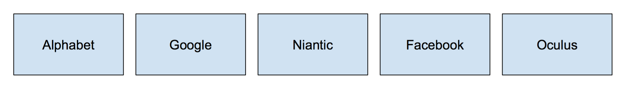
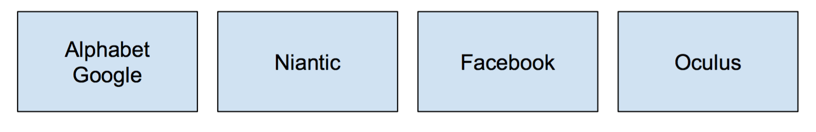
Each company is their own set with only themselves in it. A call to to find(Google) will return Google, and so forth for the remaining companies. If we were to do a call to union(Alphabet, Google), the call to find(Google) will now return Alphabet (showing that Google is a part of Alphabet).
Quick Find
For the rest of the lab, we will work with non-negative integers as the items in our disjoint sets.
One implementation you could think of is that we have each set maintain a list of the items in the set, and each item of the set hold a reference to the set that contains it.
Considering this data structure, how long would the find operation take in worst case?
|
$\Theta(1)$
|
Correct! Because each item contains a reference to the set it is contained in, we can find in constant time
|
|
|
$\Theta(\lg n)$
|
Incorrect.
|
|
|
$\Theta(n)$
|
Incorrect.
|
|
|
$\Theta(n \lg n)$
|
Incorrect.
|
|
|
$\Theta(n^2)$
|
Incorrect.
|
How about the worst case runtime of the union operation?
|
$\Theta(1)$
|
Incorrect. Think about all of the other items in the set
|
|
|
$\Theta(\lg n)$
|
Incorrect.
|
|
|
$\Theta(n)$
|
Correct! Because of we want transitive connectiveness, we must update all of the other items in the set, not just the item we pass into the union operation.
|
|
|
$\Theta(n \lg n)$
|
Incorrect.
|
|
|
$\Theta(n^2)$
|
Incorrect.
|
This list-base approach uses the quick-find algorithm, prioritizing the runtime of find operation. However, union operations are slow.
Quick Union
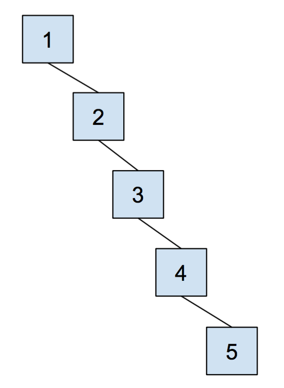
Suppose we instead prioritize making the union operation fast instead. One way we can do that is that instead of representing each set as a list, we instead represent them as a general tree. This tree will be very simple, each node only needs a reference to its parent. The root of each tree will be the face of the set it represents.
Now union is a fast $\Theta(1)$ operation, we simply need to make the root of one set into the root of another set. The cost of a quick union is that now find can now be slow. In order to find which set an item is in, we must travel to the root of the tree, which is $\Theta(N)$ in the worst case. However, we will soon see some optimizations that we can do in order to get this runtime faster.
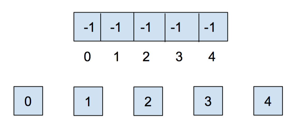
How do we actually create this data structure though? Let's take advantage of the fact that all of our items are non-negative integers. We can then use an array to keep track our sets. The indices of the array will correspond to the item itself. We will put a parent reference inside of the array. If an item does not have a parent, we will instead record the size of the set. In order to destinguish that from parent references, we will record the size $s$ of a set, as $-s$ inside of our array.
Because we are using an array as our underlying representation, we must initialize our disjoint sets with a fixed number of sets. Initially, each item is in its own set, so we will initialize all of the elements in the array to -1.
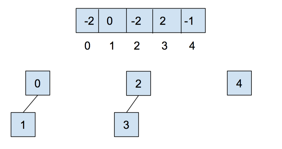
After we call union(0,1) and union(2,3), our array and our abstract representation look as below
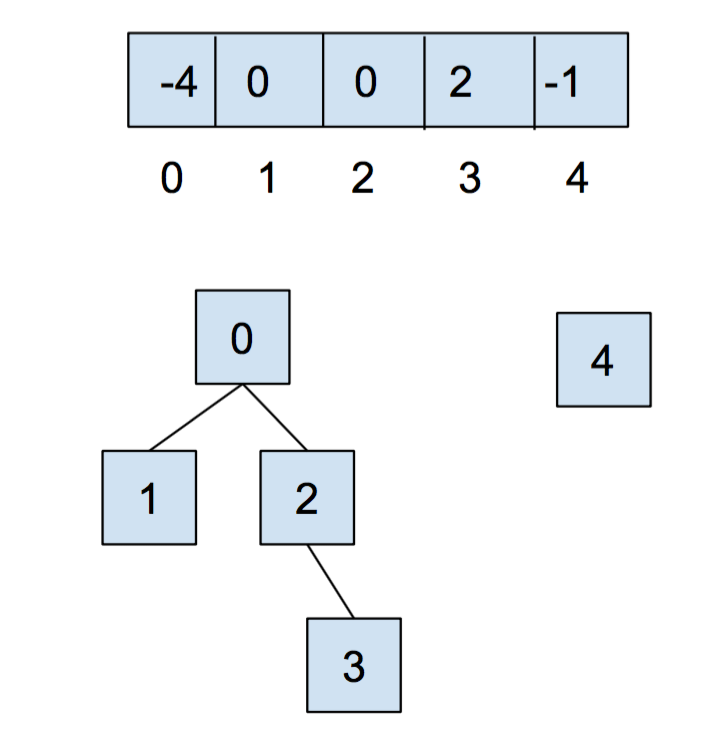
After calling union(0,2), it looks like:
Weighted Quick Union
The first optimization that we will do is called union by size. We do this in order to keep trees as shallow as possible. When we union two trees, we will make the smaller tree a subtree of the larger one, breaking ties arbitrarily.
Because we are now using union by size, the maximum depth of any item will be in $O(\lg n)$, where $n$ is the number of items stored in the data structure. Some brief intuition for this is because the depth of any element $x$ only increases when the tree $T_1$ that contains x is placed below another tree $T_2$. When that happens, the size of the tree will at least double because size($T_2) \ge$ size($T_1$). The tree that contains $x$ can only double its size at most $\lg n$ times.
Path Compression
Even though we have made a speedup with union by size, there is still yet another optimization that we can do. What would happen if we were have a tall tree and call find() repeatedly on the deepest leaf. Each time, we would have to traverse the tree from the leaf to the root. A clever optimization is to just move the leaf up so it becomes a direct child of the root. That way, the next time you call find() on that leaf, it will run much more quickly. An ever more clever idea is that we could do the same thing to every node that is on the path from the leaf to the root.
Even with path compression, the worst case runtime for find() still takes $\Theta(\lg n)$ time, however the average running time is improved substantially. Once you find an item, path compression will make finding it again faster.
The running time for any combination of $f$ find and $u$ union operations takes $\Theta(u + f \alpha(f+u,u))$ time, where $\alpha$ is an extremely slowly-growing function called the inverse Ackermann function. And by "extremely slowly-growing", I mean it grows so slowly that it's not even funny. For any practical input that you will ever use, the inverse Ackermann function will never be larger than 4 (though it can grow arbitrarily large). That means for any practical purpose (but not on any exam), a quick-union disjoint sets data structure with path compression has find operations that take constant time on average.
You can visit this link here to play around with disjoint sets.
C. Kruskal's Algorithm
Recall that we began the disjoint sets sections with the connected components problem. We'll now see how the disjoint sets can be actually used to solve the transitive connectivity problem and an application where that is needed, Kruskal's Algorithm.
Minimum Spanning Trees
Consider an undirected graph G = (V,E). A spanning tree T = (V, F) of G is tree (which if you recall is a type of graph), that contains all of the vertices of G, and |V| - 1 edges from G. Recall that in a tree, there is only one path between any any two vertices. It is possible for G to have multiple spanning trees.
If G is not a connected graph, then a similar idea is one of a spanning forest, which is a collection of trees, each having a connected component of G.
A minimum spanning tree (MST for short) T of a weighted undirected graph G, is a spanning tree where the total weight, the sum of all of the weights of the edges) is minimal. That is, no other spanning tree of G has a smaller total weight.
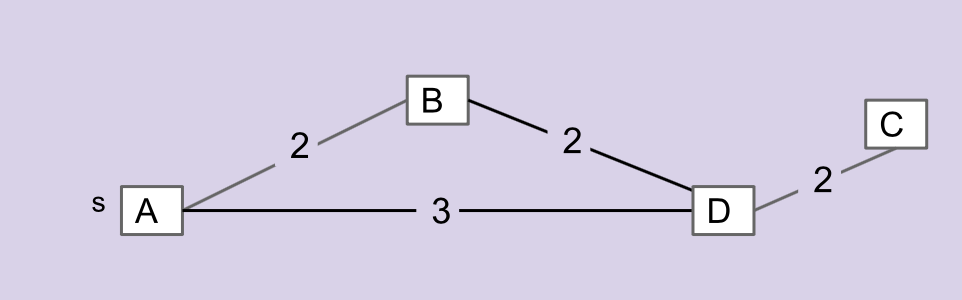
Consider the graph below. Which edges is NOT in the MST of this graph?
|
AB
|
Incorrect.
|
|
|
AD
|
Correct.
|
|
|
BD
|
Correct!
|
|
|
DC
|
Incorrect.
|
Algorithm
Kruskal's algorithm is a type of greedy algorhtm (which you will learn more about in CS170) that can calculate the MST of G. It goes as follows:
1. Create a new graph T with the same vertices as G, but no edges (yet).
2. Make a list of all the edges in G.
3. Sort the edges by weight, from least to greatest.
4. Iterate through the edges in sorted order.
 For each edge (u, w):
    If u and w are not connected by a path in T, add (u, w) to T.
Because Kruskal's algorithm never adds an edge if there is a path that already connects it, T is going to be a tree (if G is connected).
As for why Kruskal's is a minimum spanning tree, suppose we are considering a edge (u,w) to add to T, and u and w are not yet connected. Let U be all of the vertices in T that are connected so far to u and W be a set of vertices of contains everything else. This is called a cut of graph G. Let define a bridge edge or a crossing edge to be any edge that connects a vertex in U to a vertex in W. A spanning tree of G must contain at least one of these bridge edges. If we choose the bridge edge with the minimum weight, we are safe because that edge is in the MST. If there are more than one such edges, we can arbitrarily pick one. This is called the cut property.
Because we go through the edges in sorted order by weight, the edge (u,w) we are considering must have the least weight because it is the first edge we encountered.
How about the runtime of Kruskal's algorithm. As we've seen in previous labs, sorting |E| edges will take $O(|E| \lg |E|)$ time. The tricky part of Kruskal's is determining if u and w are already connected. We have seen in previous labs on how to do this. We could do a DFS or BFS starting from u and seeing if we visit w. However, if we were to do that, Kruskal's will run in worst case $\Theta(|E| |V|)$ time
But we just introduced a data structure that can find connections in almost constant time, the disjoint sets data structure. We can have the vertices of G be the items in our data structure. Whenever we add an edge (u,w) to T, we can union the sets that u and w belong in. To check if there is already a path connecting u and w, we can just call find() on both of them and see if they are part of the same set. Thus the runtime of Kruskal's is in $O(|E| \lg |E|). Note this assumes that graph creation is in constant time. If it is not, then we must take that into consideration as well.
Go here to play around with Kruskal's algorithm.
D. Implementation
For this lab, you will be implementing a naive version of Kruskal's algorithm as well as an optimized version using the Disjoint Sets data structure. You will be able to time your code using our harness in order to visually confirm that by using clever data structures, you can have remarkable increases in speed! Let's start by first pulling from skeleton, and then looking through some of the files we have.
Graph.java + Edge.java
Graph.java and Edge.java will define the Graph API we will use for this lab. It's a bit different from previous labs and so we will spend a little time discussing its implementation. In this lab, our graph will employ vertices represented by integers, and edges represented as an instance of the Edge.java. A Graph instance, maintains three instance variables.
neighborsa HashMap mapping vertices to a set of its neighboring vertices.edgesa HashMap mapping vertices to its adjacent edges.allEdgesa TreeSet of all the edges present in the current graph.
A Graph instance also has a number of instance methods that may prove useful. Read the documentation to get a better understanding of what each does!
UnionFind.java
When you open up UnionFind.java, you will see that it has a number of method headers with empty implementations. This file will hold your implementation of the Disjoint Sets data structure. Read the documentation to get an understanding of what methods need to be filled out!
Kruskal.java
Like UnionFind.java, Kruskal.java will also only have method headers initially. This file will hold your implementation of Kruskal's algorithm for calculating MSTs. For this file, you will need to implement isConnected(Graph g, int v1, int v2) which will determine if two vertices are connected using a naive algorithm such as BFS or DFS, minSpanTree(Graph g) which will hold Kruskal's algorithm using the naive implementation of isConnected and minSpanTreeFast(Graph g) which will hold Kruskal's algorithm using the Disjoint Sets data structure to efficiently determine if two vertices are connected.
Main.java
This file holds our timing harness. The harness randomly generates a graph and then runs both naive Kruskal's and optimized Kruskal's on it to calculate its MST. It will then print out the time to the command line. By default, Main.java will randomly generate a graph with 1000 vertices, however you can define how many vertices are in the graph by passing in an integer to Main.
>> javac Main.java
>> java Main.java 1337
Try running Main.java with commands growing by factors of 10 (100, 1000, 1000). What can you infer about the time as you scale the input size?
Your Task
Your task for this lab is to fully implement the methods in UnionFind.java and Kruskal.java - thus allowing Main.java to fully work. Afterwards, try running Main.java at powers of 10 to see if you see any general patterns about scale. You won't need to turn in your thoughts, but its a good exercise to on your own to solidy your understanding of Kruskal's runtime!
Testing
You'll notice that the code directory has included with it a directory named inputs. This folder contains text documents which can be read in by Graph.java to create a new graph. The syntax is as follows.
# Each line defines a new line in in the graph. The format for each line is
# fromVertex, toVertex, weight
1, 2, 3
2, 3, 2
1, 3, 1
This document creates defines a graph with three edges. One from vertex 1 to 2 with weight 3, one from 2 to 3 with weight 2, and one from 1 to 3 with weight 1. You may optionally have your text file only add vertices into the graph. This can be done by having each line contain one number representing the vertex you want to add.
# Start of the file.
1
5
3
This creates the graph with vertices 1, 5, and 3. You can define and use your own test inputs by creating a file, placing it into inputs and then reading it in using Graph.loadFromText!
E. Conclusion
Summary
Today we learned about disjoint sets and MSTs. There are other applications that disjoint sets provide (including maze generation if you want to try it). MSTs also have many usages in the real world, including connections to how the internet works.
Although we restricted ourselves to have disjoint sets with only non-negative integers as its items, we can always create an additional array that maps the integer to an Object that we actually want to be in the disjoint sets. However, for many applications, we don't care about that at all, and we care just about the ability to see if two items are in the same set.
There are also other algorithms that you can use to compute the MST, such as Prim's algorithm, which is very similar to Dijkstra's.
Submission
Push to github.