Before You Begin

The IntelliJ setup for this project differs from previous assignments. Follow the instructions carefully. Usually, if something that should be working is not working, it’s due to incomplete setup.

Your task for this project is to extend a large, existing codebase with new features. A large part of the challenge of the project is understanding the existing code and understanding what parts need to be changed, and how. Each part will require several re-readings of the spec as well as the skeleton. If you’re not sure about a part, ask before you start writing code.

We’ve generated Javadocs for the project which allows you to browse the project’s documentation online.

Pull the skeleton using the command git pull skeleton master. You’ll also need to update the library-su18 folder. You can update it by running git pull origin master inside the library-su18 directory, and if everything works as it should, you should see a collection of thousands of png files appear in the library-su18/bearmaps folder.

This project is to be done in pairs using your team repository created earlier in the semester.

Bear Maps uses Apache Maven as its build system; it integrates with IntelliJ. You will want to create a new IntelliJ project for Bear Maps. In IntelliJ, go to New -> Project from Existing Sources. Then:

1. Select your bearmaps folder, press next, and make sure to select “Import project from external model” and select Maven. Press next.
2. At the Import Project window, check: “Import Maven projects automatically”.
3. Press next until the end. If your operating system asks if IntelliJ can have permission to access your network connection, say yes.
4. It is possible that IntelliJ will not “mark” your folders correctly: Make sure to mark, if not done so already, the src/main/java directory as a sources root, the src/static directory as a sources root, and the src/test/java directory as a test sources root. To do this, right click on the folder in the explorer window (the tab on the left), and towards the bottom of the options you’ll see “Mark Directory As”.

Make sure the course javalib is not included in your project or SDK, i.e. make sure it’s not trying to use algs4.jar, etc. You will not need any of these libraries and keeping them may cause conflicts with JUnit. This also means that you cannot use any libraries outside the Java standard library and the ones already included in the project. Doing so may cause a compilation error on the autograder. Notably, we are not accommodating usage of the Princeton libraries as they are unnecessary. This project uses real world stuff only!

In case you’re curious, we’re using Maven because there are a large number of library dependencies. Rather than providing them as jar files to you with GitHub, Maven will automatically download the libraries from the internet. In larger software projects, a lot of time and effort is spent on tooling and developing an efficient development workflow. A reproducible build system like Maven makes it easy to ensure that every developer working on the project has the correct versions for all the dependencies and libraries needed to compile and run a project.

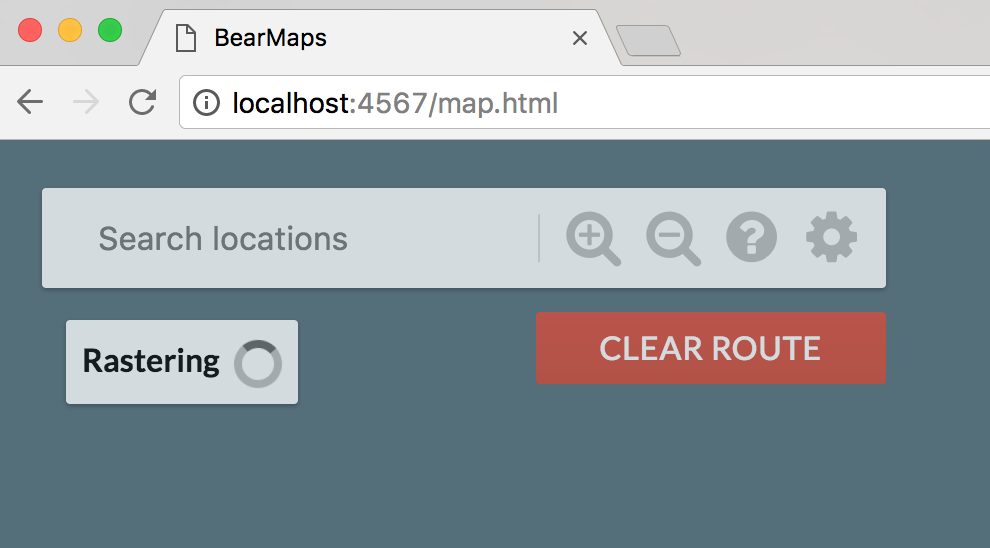
Build the project, run MapServer.java and navigate your browser (Chrome preferred; errors in other browsers will not be supported) to localhost:4567. This should load up map.html; by default, there should be a blank map. If you get a “404 Not found” error, you can open src/static/page/map.html manually by right clicking and going to Open In Browser in IntelliJ. Once you’ve opened map.html, you should see something like the window below, where the front end is patiently waiting on your back end to provide image data. Since you haven’t implemented the back end, this data will never arrive. Sad for your web browser.

If you get a 404 error, make sure you have marked your folders as described in step 4 above.

Absolutely make sure to end your instance of MapServer before re-running or starting another up. Not doing so will cause a java.net.BindException: Address already in use. If you end up getting into a situation where you computer insists the address is already in use, either figure out how to kill all java processes running on your machine (lookup how to do this online), or just reboot your computer.

Introduction

This project was originally created by former TA, Alan Yao (now at Airbnb). It is a web mapping application inspired by Alan’s time on the Google Maps team and the OpenStreetMap project, from which the tile images and map feature data was downloaded. You are working with real-world mapping data here that is freely available—after you’ve finished this project, you can even extend your code to support a wider range of features. You will be writing the back end—the web server that powers the API that the front end makes requests to.

By the end of this project, with some extra work, you can even host your application as a web app.

Meta Advice

This spec is not meant to be a comprehensive explanation of exactly how to complete the project.

Many design decisions are left to you, although suggestions are provided. Many implementation details are not given; you are expected to browse through the entirety of the skeleton (which is well-commented or self-explanatory) and learn from the comments to determine how to proceed. You will especially want to take careful note of the constants defined, such as ROOT_ULLAT.

However, the spec is written in a way so that you can proceed linearly down—that is, while each feature is partially dependent on the previous one, your design decisions, as long as they are generally reasonable, should not obstruct how you think about implementing the following parts. You are required to read the entire spec section before asking questions. If your question is answered in the spec, we will only direct you to the spec.

Last semester, Josh Hug put together a set of slides and a playlist that should help you get started. We’ve made a number of modifications to the project since last semester, but the general ideas are still the same.

Application Structure

Your job for this project is to implement the back end of a web server. To use your program, a user will open an html file in their web browser that displays a map of the city of Berkeley, and the interface will support scrolling, zooming, and route finding (similar to Google Maps). We’ve provided all of the front end code. Your code will be the back end which does all the hard work of figuring out what data to display in the web browser.

At its heart, the project works like this: The user’s web browser provides a URL to your Java program, and your Java program will take this URL and generate the appropriate output, which will displayed in the browser. For example, suppose your program were running at bloopblorpmaps.com, the URL might be:

bloopblorpmaps.com/raster&ullat=37.89&ullon=-122.29&lrlat=37.83&lrlon=-122.22&w=700&h=300

The job of the back end server (i.e. your code) is take this URL and generate an image corresponding to a map of the region specified inside the URL (more on how regions are specified later). This image will be passed back to the front end for display in the web browser.

We’ll not only be providing the front end (in the form of .html and javascript files), but we’ll also provide a great deal of starter code (in the form of .java files) for the back end. This starter code will handle all URL parsing and communication for the front end. This code uses Java Spark as the server framework. You don’t need to worry about the internals of this as our code handles all the messy translation between web browser and your Java programs.

Overview

You will implement three required classes for this project, in addition to any helper classes that you decide to create. These three classes are Rasterer, GraphDB, and Router. They are described very briefly below. More verbose descriptions follow.

The Rasterer class will take as input an upper left latitude and longitude, a lower right latitude and longitude, a window width, and a window height. Using these six numbers, it will produce a 2D array of filenames corresponding to the files to be rendered. Historically, this has been the hardest task to fully comprehend and most time consuming part of the project.

The GraphDB class will read in the OpenStreetMap dataset and store it as a graph. Each node in the graph will represent a single intersection, and each edge will represent a road. How you store your graph is up to you. This will be the strangest part of the project, since it involves using complex real world libraries to process complex real world data.

The Router class will take as input a GraphDB, a starting latitude and longitude, and a destination latitude and longitude, and it will produce a list of nodes (i.e. intersections) that you get from the start point to the end point.

Warning: Unlike prior assignments in your CS classes, we’ll be working with somewhat messy real world data. This is going to be frustrating at times, but it’s an important skill and something that we think will serve you well moving forwards.

The biggest challenges in this assignment will be understanding what rastering is supposed to do, as well as figuring out how to parse XML files for GraphDB.

In the src/test/java folder, we’ve provided some client side JUnit tests that you can run for each part. Make sure to use this to drive your development process.

Testing

The src/test/java file contains six test files. These tests are to help save you time. In an ideal world, we’d have more time to get you to write these tests yourself so that you’d deeply understand them, but we’re giving them to you for free. You should avoid leaning too heavily on these tests unless you really understand them! The staff will not explain individual test failures that are covered elsewhere in the spec, and you are expected to be able to resolve test failures using the skills you’ve been learning all semester to effectively debug.

Ineffective/inappropriate strategies for debugging

Running the JUnit tests over and over again while making small changes each time, staring at the error messages and then posting on Piazza asking what they mean rather than carefully reading the message and working to understand it.

Effective strategies include

• Using the debugger.
• Reproducing the buggy inputs in a simpler file that you write yourself.
• Rubber ducky debugging.

You can feel free to modify these files however you want. We will not be testing your code on the same data as is given to you for your local testing—thus, if you pass all the tests in this file, you are not guaranteed to pass all the tests on the actual autograder.

These tests should be mostly self-explanatory. If you’re failing routing tests, make sure you’re passing all graph building tests, since your router will almost certainly fail if your graph is not working.

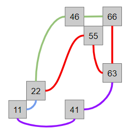
The tiny versions of the graph builder test and router test are on a graph so small that you can draw it out by hand and even compute the results of the routing queries by eye. This graph is depicted below (lat and lon not show). Each edge in the image represents a different way (colors picked such that they should appear distinct, so long as you are not 100% achromatopsic). See tiny-clean.osm.xml in library-su18/bearmaps for the full details.

We’ve also provided html test files, test.html, testTwelveImages.html, and test1234.html that you can use to test your project without using the front end. These files make a /raster API call and draws the result. You can modify the query parameters in these files. These files allow you to make a specific call easily.

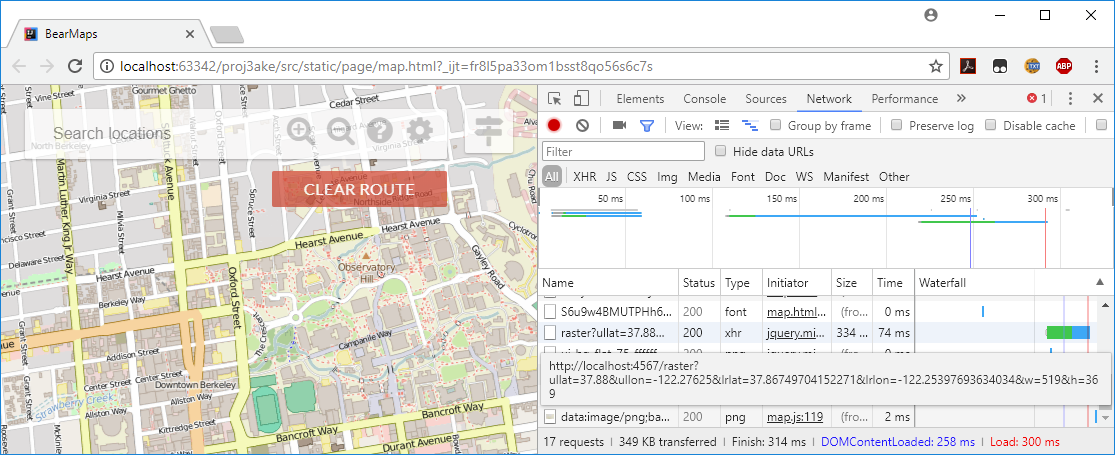
If you want to debug using map.html, you may find your browser’s Javascript console handy: on Windows, in Chrome you can press F12 to open up the developer tools, click the network tab, and all calls to your MapServer should be listed under type xhr, and if you mouse-over one of these xhr lines, you should see the full query appear, for example (click for higher resolution):

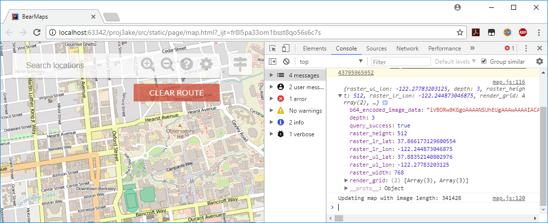
You can also see the replies from your MapServer in the console tab.

Map Rastering

Rastering is the job of converting information into a pixel-by-pixel image. In the Rasterer class you will take a user’s desired viewing rectangle and generate an image for them.

Implement the Rasterer class by completing the getMapRaster method.

public RasterResultParams getMapRaster(RasterRequestParams params)

The user’s desired input will be provided to you as a RasterRequestParams object. The goal of your rastering code is to create a RasterResultParams object containing the correct response so that the browser will know what image to render on the screen.

The most challenging part of this process is computing the renderGrid, a String[][] that corresponds to the files that should be displayed in response to this query.

Example Query

As a specific example (given as testTwelveImages.html in the skeleton files), the user might specify that they want the following information:

{lrlon=-122.2104604264636, ullon=-122.30410170759153, w=1085.0, h=566.0, ullat=37.870213571328854, lrlat=37.8318576119893}

This means that the user wants the area of Earth delineated by the rectangle between longitudes -122.2104604264636 and -122.30410170759153 and latitudes 37.870213571328854 and 37.8318576119893, and that they’d like them displayed in a window roughly 1085 x 566 pixels in size. We call the user’s desired display location on Earth the query box.

To display the requested information, we need street map pictures, which we’ve provided in library-su18. All of the images provided are 256 x 256 pixels, but they differ in that each image shows a different region of the map at a particular level of zoom.

• d0_x0_y0.png is the entire map, and covers the entire region.
• d1_x0_y0.png, d1_x0_y1.png, d1_x1_y0.png, and d1_x1_y1.png are also the entire map, but together cover the same space at double the resolution. d1_x0_y0 is the northwest corner of the map, d1_x1_y0 is the northeast corner, d1_x0_y1 is the southwest corner, and d1_x1_y1 is the southeast corner.

More generally, at the $D$th level of zoom, there are $4^D$ images, with names ranging from dD_x0_y0 to dD_xk_yk, where $k$ is $2^D - 1$. As $x$ increases from $0$ to $k$, we move eastwards, and as $y$ increases from $0$ to $k$, we move southwards.

The job of your rasterer class is decide, given a user’s query, which files to serve up. For the example above, your code should return the following 2D array of strings:

[[d2_x0_y1.png, d2_x1_y1.png, d2_x2_y1.png, d2_x3_y1.png],
[d2_x0_y2.png, d2_x1_y2.png, d2_x2_y2.png, d2_x3_y2.png],
[d2_x0_y3.png, d2_x1_y3.png, d2_x2_y3.png, d2_x3_y3.png]]

This means that the browser should display d2_x0_y1.png in the top left, then d2_x1_y1.png to the right of d2_x0_y1.png, and so forth. Thus our “rastered” image is actually a combination of 12 images arranged in 3 rows of 4 images each.

Our MapServer code will take your 2D array of strings and display the appropriate image in the browser. If you’re curious how this works, see the renderImage method in the MapServer class.

Computing the renderGrid

Since each image is 256 x 256 pixels, the overall image given above will be 1024 x 768 pixels. There are many combinations of images that cover the query box. For example, we could instead use higher resolution images of the exact same areas of Berkeley. For example, instead of using d2_x0_y1.png, we could have used d3_x0_y2.png, d3_x1_y2.png, d3_x0_y3.png, d3_x1_y3.png while also substituting d2_x1_y1.png by d3_x2_y2.png, d3_x3_y2.png, etc. The result would be total of 48 images arranged in 6 rows of 8 images each (make sure this makes sense!). This would result in a 2048 x 1536 pixel image.

You might be tempted to say that a 2048 x 1536 image is more appropriate than 1024 x 768. After all, the user requested 1085 x 556 pixels and 1024 x 768 is too small to cover the request in the width direction. However, pixel counts are not the way that we decide which images to use.

Instead, to rigorously determine which images to use, we will define the longitudinal distance per pixel (lonDPP) as follows: Given a query box or image, the lonDPP of that box or image is

$$\texttt{lonDPP} = \frac{\text{lower right longitude} - \text{upper left longitude}}{\text{width of the image (or box) in pixels}}$$

For example, for the query box in the example in this section:

$$\texttt{lonDPP} = \frac{-122.2104604264636 + 122.30410170759153}{1085} \approx 8.63 \times 10^{-5}$$

At Berkeley’s latitude, this is very roughly 25 feet of distance per pixel.

The images that you return as a String[][] when rastering must be those that:

• Include any region of the query box.
• Have the greatest lonDPP that is less than or equal to the lonDPP of the query box (as zoomed out as possible). If the requested lonDPP is less than what is available in the data files, you should use the lowest lonDPP available instead (i.e. the images at the deepest level).

Let’s consider the following tiles from different image depths. Our goal is to find the tiles with the greatest lonDPP that is still less than the lonDPP requested by the query box.

Image depth 1 (ex. d1_x0_y0)

Every tile has lonDPP equal to $1.72 \times 10^{-4}$. (For an explanation of why, see the next section.) This is greater than the lonDPP of the query box, and is thus unusable. This makes intuitive sense: If the user wants an image which covers roughly 25 feet per pixel, we shouldn’t use an image that covers about 50 feet per pixel because the resolution is too poor.

Image depth 2 (ex. d2_x0_y1)

The lonDPP is $8.58 \times 10^{-5}$, which is better (more detailed) than the user requested, so this is fine to use.

Image depth 3 (ex. d3_x0_y2.png)

The lonDPP is $4.29 \times 10^{-5}$. This is also smaller than the desired lonDPP, but using it is overkill since depth 2 tiles are already good enough.

It can be helpful to think of lonDPP as blurriness. The d0 image is the blurriest (most zoomed out or highest lonDPP), and the d7 images are the sharpest (most zoomed in with the lowest lonDPP).

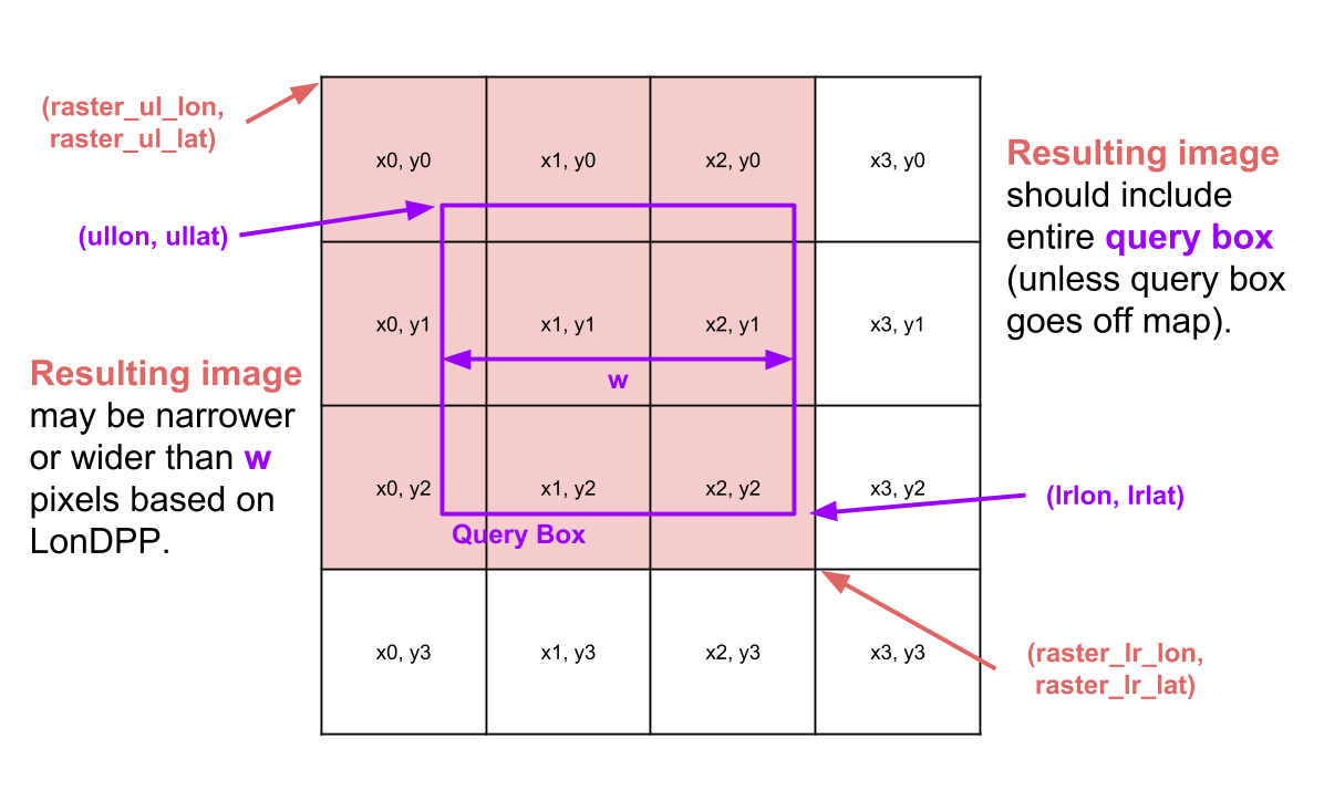
As an example of an intersection query, consider the image below, which summarizes key parameter names and concepts. In this example search, the query box intersects 9 of the 16 tiles at depth 2.

One natural question is: Why not use the best quality images available, the ones with the smallest lonDPP?

The technical answer is that the front end doesn’t do any rescaling, so if we used ultra low lonDPP values for all queries, we’d end up with absolutely gigantic images displayed in our web browser.

From a user interface perspective, each level’s images introduce more and more details that aren’t necessarily present farther away. It’s arguably more understandable for the user to hide these details so they aren’t overwhelmed by all the zoomed-in map details.

File Display Demo

For an interactive demo of how the provided images are arranged, try the following file display demo. Try typing in a filename (.png extension is optional), and it will show what region of the map this file corresponds to, as well as the exact coordinates of its corners, in addition to the lonDPP in both longitude units per pixel and feet per pixel.

Your browser does not support the HTML5 canvas tag.

File display demo

Field	Value
ullon
ullat
lrlon
lrlat
lonDPP
feetDPP

Image File Layout and Bounding Boxes

There are four constants that define the coordinates of the world map, all given in MapServer.java. The first is ROOT_ULLAT, which tells us the latitude of the upper left corner of the map. The second is ROOT_ULLON, which tells us the longitude of the upper left corner of the map. Similarly, ROOT_LRLAT and ROOT_LRLON give the latitude and longitude of the lower right corner of the map. All of the coordinates covered by a given tile are called the “bounding box” of that tile. So for example, the single depth 0 image d0_x0_y0 covers the coordinates given by ROOT_ULLAT, ROOT_ULLON, ROOT_LRLAT, and ROOT_LRLON.

Recommended exercise: Try opening d0_x0_y0.png. Then, use Google Maps to show the point given by ROOT_ULLAT, ROOT_ULLON. You should see that this point is the same as the top left corner of d0_x0_y0.png.

Another important constant in MapServer is TILE_SIZE. This is important because we need this to compute the lonDPP of an image file. For the depth 0 tile, the lonDPP is just (ROOT_LRLON - ROOT_ULLON) / TILE_SIZE, i.e. the number of units of longitude divided by the number of pixels.

All levels in the image library cover the exact same area. So for example, d1_x0_y0.png, d1_x1_y0.png, d1_x0_y1.png, and d1_x1_y1.png comprise the northwest, northeast, southwest, and southeast corners of the entire world map with coordinates given by the ROOT_ULLAT, ROOT_ULLON, ROOT_LRLAT, and ROOT_LRLON parameters.

The bounding box given by an image can be mathematically computed using the information above. For example, suppose we want to know the region of the world that d1_x1_y1.png covers. We take advantage of the fact that we know that d0_x0_y0.png covers the region between longitudes -122.29980468 and -122.21191406 and between latitudes 37.82280243 and 37.89219554. Since d1_x1_y1.png is just the southeastern quarter of this region, we know that it covers the region between longitudes -122.25585937 and -122.21191406 and between latitudes 37.82280243 and 37.85749898.

Similarly, we can compute the lonDPP in a similar way. Since d1_x1_y1.png is 256 x 256 pixels (as are all image tiles), the lonDPP is,

$$\texttt{lonDPP} = \frac{-122.21191406 - -122.25585937}{256} \approx 1.72 \times 10^{-4}$$

If you’ve fully digested the information described in the spec so far, you now know enough to figure out which files to provide given a particular query box. See the slides and playlist for more hints if you’re stuck.

Corner Cases

The query window shown above corresponds to the viewing window in the client. Although you are returning a full image, it will be translated (with parts off the window) appropriately by the client.

You may end up with an image, for some queries, that ends up not filling the query box and that is okay. This arises when your latitude and longitude query do not intersect enough tiles to fit the query box. You can imagine this happening with a query very near the edge (in which case you just don’t collect tiles that go off the edge); a query window that is very large, larger than the entire dataset itself; or a query window in lat and lon that is not proportional to its size in pixels. See the slides for an example of a query window whose width/height is not proportional to lat/lon.

You can also imagine that the user might drag the query box to a location that is completely outside of the root longitude/latitudes. In this case, there is nothing to raster, raster_ul_lon, raster_ul_lat, etc. are arbitrary, and return RasterResultParams.queryFailed(). If the server receives a query box that doesn’t make any sense, like if ullon, ullat is located to the right of lrlon, lrlat, you should also return RasterResultParams.queryFailed().

Rastering Runtime

Your constructor should take time linear in the number of tiles that match the query.

You may not iterate through or explore all tiles to search for intersections. Suppose there are $k$ tiles intersecting a query box, and $N$ tiles total. Your entire query should run in $O(k)$ time. Your algorithm should not run in $\Theta(N)$ time. This is not for performance reasons, since $N$ is going to be pretty small in the real world (less than tens of thousands), but rather because the $\Theta(N)$ algorithm is inelegant.

The autograder is not smart enough to tell the difference, so if you really insist, you can do the $\Theta(N)$ algorithm. But we encourage you to try to figure out something better.

Graphs & Map Data

In this part of the project, you’ll use a real world dataset combined with an industrial strength dataset parser to construct a graph. This is similar to tasks you’ll find yourself doing in the real world, where you are given a specific tool and a dataset to use, and you have to figure out how they go together. It’ll feel shaky at first, but once you understand what’s going on it won’t be so bad.

Routing and location data is provided to you in the berkeley.osm file. This is a subset of the full planet’s routing and location data. The data is presented in the OSM XML file format.

XML is a markup language for encoding data in a document. Open up the berkeley.osm file for an example of how it looks. Each element looks like an HTML tag, but for the OSM XML format, the content enclosed is (optionally), more elements. Each element has attributes, which give information about that element, and sub-elements, which can give additional information and whose name tell you what kind of information is given.

The first step of this part of the project is to build a graph representation of the contents of berkeley.osm. We have chosen to use a SAX parser, which is an “event-driven online algorithm for parsing XML documents”. It works by iterating through the elements of the XML file. At the beginning and end of each element, it calls the startElement and endElement callback methods with the appropriate parameters.

Your job will be to override the startElement and endElement methods so that when the SAX parser has completed, you have built a graph. Understanding how the SAX parser works is going to be tricky.

You will find the documentation for GraphDB and GraphBuildingHandler helpful, as well as the example code in GraphBuildingHandler.java, which gives a basic parsing skeleton example. There is an example of a completed handler in the src/main/java/example folder called CSCourseDBHandler.java that you might find helpful to look at.

Read through the OSM wiki documentation on the various relevant elements:

• Tags
• Highway keys
• Way elements
• Node elements

You will need to use all of these elements, along with their attribute’s values, to construct your graph for routing.

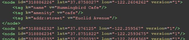
The node, pictured above, comprises the backbone of the map; the lat, lon, and id are required attributes of each node. They may be anything from locations to points on a road. If a node is a location, a tag element, with key “name” will tell you what location it is—above, we see an example.

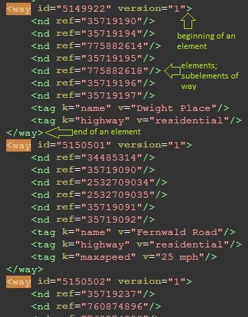
The way, pictured above, is a road or path and defines a list of nodes, with name nd and the attribute ref referring to the node id, all of which are connected in linear order. Tags in the way will tell you what kind of road it is—if it has a key of “highway”, then the value corresponds to the road type. See the Javadoc on ALLOWED_HIGHWAY_TYPES for restrictions on which roads we care about.

You should ignore all one-way tags and pretend all roads are two-way. (This means your directions are not safe to use, but there are some inaccuracies in the OSM data anyway).

Part of your job will be decide how to store the graph itself in your GraphDB class. Note that the final step of graph construction is to “clean” the graph and destroy all nodes that are disconnected. Your GraphDB will need to permit the insertion and deletion of nodes.

Note: You don’t need to actually store the maxSpeed anywhere since we ignore the speed limits when calculating the route. We’ve provided this in the skeleton in case you want to play around with this, but unfortunately the provided data set is missing a bunch of speed limits so it didn’t turn out to be particularly useful.

Route Search

For the final required part of this project, we want to compute the shortest path between any two points clicked on the map.

The web browser will send us four values: the start point’s longitude and latitude, and the end point’s longitude and latitude. Implement shortestPath in your Router class so that it computes the single-pair shortest path and satisfies the requirements in the documentation.

Your route should be the shortest path that starts from the closest connected node to the start point and ends at the closest connected node to the endpoint. Implement the closest method in the GraphDB class to compute the closest connected node to a given longitude and latitude. For now, the linear time algorithm is acceptable. Later in the project, we’ll implement an optimization to significantly improve the runtime of closest.

Distance between two nodes is defined as the great-circle distance between their two points (lon1, lat1) and (lon2, lat2). The length of a path is the sum of the distances between the ordered nodes on the path. We do not take into account driving time (speed limits). Use the distance method that we’ve defined to compute the distance between any two (lon, lat) coordinate pairs.

In the real-world, we often prefer to reuse implementations provided by the Java standard library or third-party libraries. But another useful skill to develop as a programmer is the skill of taking pseudocode, or a high-level description of the algorithm, and turning it into a real program that works together with the rest of our implementation. For this part of the project, we ask you to implement existing algorithms given standard pseudocode found online.

A* Search

Let $d$ be the distance between the start and end node. You cannot explore all nodes within distance $d$ from the start node and expect to pass the autograder (for long paths, this could be more than half the nodes in the map).

While Dijkstra’s algorithm for finding shortest paths works well, in practice if we can, we use A* search. Dijkstra’s algorithm is a single-source shortest paths algorithm which visits all nodes at a distance $d$ or less from the start node. However, in cases like this where we know the direction that we should be searching in, we can employ that information as a heuristic and solve a smaller problem called, single-pair shortest paths.

Let $n$ be some node on the search fringe (a min-priority queue), $s$ be the start node, and $t$ be the destination node. A* differs from Dijkstra’s in that it uses a heuristic $h(n)$ for each node $n$ that tells us how close it is to $t$. The priority associated with $n$ should be $f(n) = g(n) + h(n)$, where $g(n)$ is the shortest known path distance from $s$ and $h(n)$ is the heuristic distance, the great-circle distance from $n$ to $t$, and thus the value of $h(n)$ should shrink as $n$ gets closer to $t$. This helps prevent the algorithm from exploring too far in the wrong direction.

This amounts to only a small change in code from the Dijkstra’s version (for us, one line).

See Josh Hug’s Routing Coding Tips for an introduction to solving the A* routing problem, and some of the subtleties involved in different student implementations of A* search.

If you find yourself stuck debugging the shortest path for more than hour, we suggest starting over from scratch. Many shortest paths bugs require thinking through particular edge cases. It’s often faster to rewrite the program, and then compare the differences between the implementations and how they treat visited and unvisited nodes.

Nearest Neighbor Search

You already have a naive implementation for the closest method in GraphDB which returns the id for the node closest to the given coordinates based on great-circle distance. Given a graph with $N$ nodes, this results in a $\Theta(N)$ time algorithm as it needs to loop over all the nodes in the graph just to find a single nearest neighbor, or the closest connected node.

To improve runtime, we will be implementing a k-d tree which will allow us to search for the nearest neighbor to a clicked point in (typically) $\Theta(\log N)$ time. The drawback is that we will need to construct the tree in $\Theta(N \log N)$ time. Even with this upfront cost to constructing the tree, this is an overall improvement over the naive algorithm since we only need to construct the k-d tree once, but we can query it as many times as we want in logarithmic time. This makes sense for our web app as one instance of the app can run for a very long time and handle thousands if not millions (or billions) of nearest neighbor search requests.

k-d Tree

Implement a new k-d tree class using the pseudocode and algorithms as described on Wikipedia. Because we have all of our data upfront and our data doesn’t change, we only need to implement k-d tree Construction and Nearest Neighbor Search. Once completed, replace the naive implementation of closest with a call to your k-d tree.

You might find the lecture slides on constructing a k-d tree helpful. For a demonstration of nearest neighbor search on a k-d tree, see the 2D Tree Demo by Robert Sedgewick and Kevin Wayne.

‘Intersecting the splitting hyperplane and hypersphere’ in the 2-dimensional case refers to the splitting lines and distance circles in the demo.

Working in 2-D

Because the standard k-d tree data structure assumes a flat, 2-dimensional grid of points (Euclidean geometry), we will need to apply a few modifications so that it works with our spherical model of the Earth. Fortunately, we’ve done the research for you. There are a number of ways to solve this problem in the general setting, but we suggest projecting each coordinate pair to a 2-D grid centered on Berkeley and then computing the nearest neighbors using the k-d tree in this $(x, y)$ space.

We’ve provided a few methods to projectToX and projectToY that do all the work of converting latitudes and longitudes to $(x, y)$ points for you. Make sure all computations in the k-d tree operate on $(x, y)$ points, not latitudes and longitudes.

In the k-d tree’s $(x, y)$ space, we can compute the straightline distance between any two points using the Euclidean distance formula.

static double euclidean(double x1, double x2, double y1, double y2) {
    return Math.sqrt(Math.pow(x1 - x2, 2) + Math.pow(y1 - y2, 2));
}

Note that this method won’t work on latitudes and longitudes. For those, use the great-circle distance method instead.

While this approach is extremely accurate for small areas of Earth, it doesn’t scale well outside of the geographic region spanning the Bay Area as the projection gets increasingly distorted the further away we get from Berkeley. For a more general solution, the common recommendation is to convert the coordinate points to points in 3-dimensional space with the origin centered on Earth, but this requires a more complex k-d tree implementation and could potentially be harder to debug.

Location Search

In the Autocomplete lab, we will be implementing a trie to allow for fast prefix searches. This part won’t be tested or included in the grading for the main portion of the project.

Locations

In the berkeley.osm file, we consider all nodes with a name tag a location. This name is not necessarily unique and may contain things like road intersections.

Autocomplete

We would like to implement an autocomplete system where a user types in a partial query string, like “Mont”, and is returned a list of locations that have “Mont” as a prefix. To do this, implement getLocationsByPrefix, where the prefix is the partial query string. The prefix will be a cleaned name for search that is:

1. Everything except characters A through Z and spaces removed.
2. Everything is lowercased.

The method will return a list containing the full names of all locations whose cleaned names share the cleaned query string prefix, without duplicates.

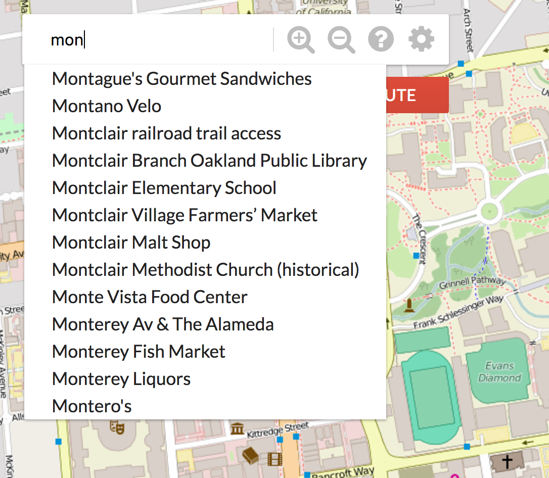
Using a trie, we can traverse to the node that matches the prefix (if it exists) and then collect all valid words that are a descendant of that node.

Assuming that the lengths of the names are bounded by some constant, querying for prefix of length $s$ should take $O(k)$ time where $k$ is the number of words sharing the prefix.

Location Search

The user should also be able to search for places of interest. Implement getLocations which collects a List<LocationParams> containing information about the matching locations—that is, locations whose cleaned name match the cleaned query string exactly. This is not a unique list and should contain duplicates if multiple locations share the same name (i.e. Top Dog, Bongo Burger). See the Javadocs and the LocationParams class for more information.

Implementing this method correctly will allow the web application to draw red dot markers on each of the matching locations. Note that because the location data is not very accurate, the markers may be a bit off from their real location. For example, the west side Top Dog is on the wrong side of the street!

Suppose there are $k$ results. Your query should run in $O(k)$.

Optional: Possible Extensions

Turn-by-turn Navigation

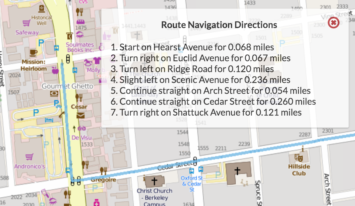
As an optional feature, you can use your A* search route to generate a sequence of navigation instructions that the server will then be able to display when you create a route. To do this, implement the additional method routeDirections in your Router class. This part of the project is not worth any points (even gold points), but it is awfully cool.

How we will represent these navigation directions will be with the NavigationDirection object defined within Router.java. A direction will follow the format of “DIRECTION on WAY for DISTANCE miles”. Note that “DIRECTION” is an int that will correspond to a defined String direction in the directions map, which has 8 possible options:

• “Start”
• “Continue straight”
• “Slight left/right”
• “Turn left/right”
• “Sharp left/right”

To minimize the amount of String matching you will need to do to pass the autograder, we have formatted the representation for you. You will simply have to set the correct “DIRECTION”, “WAY”, and “DISTANCE” values for the given direction you want when creating a NavigationDirection.

What direction a given NavigationDirection should have will be dependent on your previous node and your current node along the computed route. Specifically, the direction will depend on the relative bearing between the previous node and the current node, and should be as followed:

• Between -15 and 15 degrees the direction should be “Continue straight”.
• Beyond -15 and 15 degrees but between -30 and 30 degrees the direction should be “Slight left/right”.
• Beyond -30 and 30 degrees but between -100 and 100 degrees the direction should be “Turn left/right”.
• Beyond -100 and 100 degrees the direction should be “Sharp left/right”.

The navigation will be a bit complicated due to the fact that the previous and current node at a given point on your route may not necessarily represent a change in way. As a result, what you will need to do as you iterate through your route is determine when you do happen to change ways, and if so generate the correct distance for the NavigationDirection representing the way you were previously on, add it to the list, and continue. If you happen to change ways to one without a name, it’s way should be set to the constant “unknown road”.

As an example, suppose when calling routeDirections for a given route, the first node you remove is on the way “Shattuck Avenue”. You should create a NavigationDirection where the direction corresponds to “Start”, and as you iterate through the rest of the nodes, keep track of the distance along this way you travel. When you finally get to a node that is not on “Shattuck Avenue”, you should make sure NavigationDirection should have the correct total distance travelled along the previous way to get there (suppose this is 0.5 miles). As a result, the very first NavigationDirection in your returned list should represent the direction “Start on Shattuck Avenue for 0.5 miles.”. From there, your next NavigationDirection should have the name of the way your current node is on, the direction should be calculated via the relative bearing, and you should continue calculating its distance like the first one.

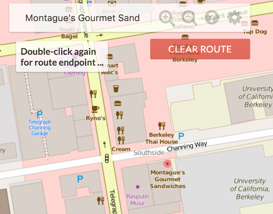
After you have implemented this properly you should be able to view your directions on the server by plotting a route and clicking on the button on the top right corner of the screen.

Front End Integration

Currently, you raster the entire image and then pass it to the front end for display, and re-raster every call. A better approach, and the one that popular rastering mapping applications nowadays take, would be to simply pass each tile’s raster to the front end, and allow the front end to assemble them on the page dynamically. This way, the front end can make the requests for the image assets and cache them, vastly reducing repetitive work when drawing queries, especially if they use tiles that have already been drawn before.

Likewise, the front end could handle route drawing as all the back end needs to pass to the front end are the points along the route.

However, this poses a major problem to the project’s design—it overly simplifies the amount of work you need to do and moves a large amount of the interesting work to the front end, so for this small project you implement a simplified version.

Vectored Tiles

While for this project we’ve provided the mapping data in the form of images per tile, in reality these images are rastered from the underlying vector geometry—the roads, lines, filled areas, buildings and so on that make up the tile. These can all be drawn as triangles using a rendering API like OpenGL or WebGL; this speeds up the process even more, as much of the work is now passed on to the GPU which can handle this far more efficiently than the CPU. This data is all available from the OpenStreetMap vector tileset if you want to pursue this route of action. However, doing so is far beyond the scope of the course and more along the lines of CS 184.

3-d Tree with ECEF coordinates

In many real-world mapping applications, we can’t assume that the only region of interest is the area surrounding Berkeley. Our current approach for the k-d tree data structure projects latitudes and longitudes on a sphere out onto a 2-dimensional $(x, y)$ grid centered on Berkeley. While this works well for the area around Berkeley, the projection distorts distances so much that it becomes practically useless when used to map outside the area of California.

Given that k-d trees work in Euclidean space, the solution is to model points on the sphere using full, 3-dimensional geometry and using a 3-d tree. This requires converting each latitude and longitude coordinate pair to Earth-Centered, Earth-Fixed coordinates and computing the nearest neighbor using the Euclidean distance between points in 3-dimensions. This will more accurately model the relative distances between points on a sphere, though better models will want to take into account variations in elevation and the fact that the Earth is not perfectly spherical.

Speed of Travel

Not all roads enforce the same speed limits: residential streets with stop signs are much slower than boulevards and avenues with street lights, which are usually slower than highways. Our current routing algorithm only takes into account the exact distance but not the speed of travel along each path. This isn’t too hard to incorporate, but our mapping dataset is too incomplete to take full advantage of it.

Better navigation solutions can also incorporate real-time data to determine slowdowns and traffic patterns. Google Maps, for example, uses real-time data from users and traffic agencies to determine slowdowns and then re-route based on all available traffic data at the time of the request.

FAQ

If your question is for debugging help, you must be prepared to explain the error that is being caused and have a test or input that can easily reproduce the bug for ease of debugging. If you come to us saying something does not work, but have not written any tests or attempted to use the debugger, we will not help you.

When we do provide debugging help, it may be at a high level, where we suggest ways to reorganize your code in order to make clarity and debugging easier. It is not a good use of your time or the TAs’ time to try to find bugs in something that is disorganized and brittle.

I pass all the local tests, but I’m getting a NoSuchElementException in the

autograder

The autograder uses randomized sources and targets. Some targets may not be reachable from all sources. In these cases, you can do anything you want (like return an empty list of longs) except let your program crash.

My router isn’t working and I’m having a really hard time debugging. Do you

have any suggestions?

Debugging routing is very tough since you only see the end result of the entire process and don’t have a good sense of what got enqueued.

Some common issues include:

• Not handling the case where the target isn’t reachable (see above).
• Casting priorities as integers.
• Setting distTo values that stick around between calls to shortestPath.
• Using static variables where instance or local variables are more appropriate. There is no reason to have any static variables.
• Marking nodes when adding to the fringe when using approach 2 or 3. You should only mark nodes when you take them out.
• Broken comparators that don’t handle cases like where two items are equal.
• Not overriding hashCode and/or equals for custom objects stored in a collection like a Map, Set, or List.
• Try the Code Inspection feature in IntelliJ. Click Analysis -> Inspect Code, then click OK. Look under “Probable Bugs”. This is a list of pieces of code that IntelliJ considers to be possible buggy. IntelliJ is not that smart, however, and not all of these will be actual bugs. However, we hope the list will give you a few places to look. You can make the “Inspect Code” feature even more powerful by importing the provided library-su18/inspections.xml using File -> Import Settings.
• Don’t use recursion for A*. Java doesn’t do any sort of tail call optimization, and thus can’t handle deep recursion.

If all else fails, start this part again from scratch. Debugging 30 lines of code for 10 hours is not a good use of your time, and subtle bugs can be very tough to detect. Might be easier to do a clean restart, especially if you think you have a solid understanding of A*. If you don’t have a strong understanding of A*, it’s probably best to review the Routing Coding Tips.

My initial map doesn’t fill up the screen!

If your monitor resolution is high and the window is fullscreen, this can happen. Refer to the reference solution to see if yours looks similar.

In the browser, zooming out only appears to shift the map, and I’m confident my

rastering code is correct

If you click on the gear icon, check the box for “Constrain map dimensions”. This issue is due to the window size being too large which sometimes causes the front end to handle zooming out poorly. Alternately, try making your browser window smaller. Also make sure you’re allowing all the rastering to finish (sometimes the front end calls raster a couple more times to get the result of the zoom just right).

I don’t draw the entire query box on some inputs because I don’t intersect

enough tiles.

That’s fine, that’ll happen when you go way to the edge of the map. For example, if you go too far west, you’ll never reach the bay because it does not exist.

I’m getting funky behavior with moving the map around, my image isn’t large

enough at initial load, after the initial load, I can’t move the map, or after

the initial load, I start getting NaN as input params.

These all have to do with your returned parameters being incorrect. Make sure you’re returning the exact parameters as given in the slides or the test html files.

I sometimes pass the timing tests when I submit, but not consistently.

If you have a efficient solution: it will always pass. I have yet to fail the timing test with either my solution or any of the other staff’s solutions over a lot of attempts to check for timing volatility.

If you have a borderline-efficient solution: it will sometimes pass. That’s just how it is, and there really isn’t any way around this if we want the autograder to run in a reasonable amount of time.

How do query boxes or bounding boxes make sense on a round world?

For the rastering part of the project, we assume the world is effectively flat on the scale of the map you’re looking at. In truth, each image doesn’t cover a rectangular area, but rather a “spherical cap”.

I’m suddenly having compilation issues.

First, make sure you haven’t imported any of the usual libraries. If you have algs4.jar or any of the usual javalib stuff in your project, things can go terribly wrong with error messages that are totally useless.

I’m missing xml files and/or library-su18 is not updated.

Go into the library-su18 directory and try the commands git submodule update --init followed by git checkout master.

Submission

You need only submit the src folder. It should retain the structure given in the skeleton. Do not submit or upload to git your osm or test files. Attempting to do so will eat your internet bandwidth and hang your computer, and will waste a submission.

Do not make your program have any maven dependencies other than the ones already provided. Doing so may fail the autograder.

Acknowledgements

Data made available by OSM under the Open Database License.

JavaSpark web framework and Google Gson library.

Alan Yao for creating the original version of this project.