
FAQ #
Each assignment will have an FAQ linked at the top. You can also access it by adding “/faq” to the end of the URL. The FAQ for Lab 21 is located here.
Introduction #
As usual, pull the files from the skeleton and make a new IntelliJ project.
In yesterday’s lab, you were introduced to several comparison sorting algorithms: namely, selection sort, insertion sort, and heap sort. In this lab, we will continue our discussion of comparison-based sorts with merge sort and quicksort.
Here is a nice visualizer for all of the sorts we covered yesterday and will cover today.
New Idea: “Divide and Conquer” #
The first few sorting algorithms we’ve previously introduced work by iterating through each item in the collection one-by-one. With insertion sort and selection sort, both maintain a “sorted section” and an “unsorted section” and gradually sort the entire collection by moving elements over from the unsorted section into the sorted section. Another approach to sorting is by way of divide and conquer. Divide and conquer takes advantage of the fact that empty collections or one-element collections are already sorted. This essentially forms the base case for a recursive procedure that breaks the collection down into smaller pieces before merging adjacent pieces to form a completely sorted collection.
The idea behind divide and conquer can be broken down into the following 3-step procedure.
- Split the elements to be sorted into two collections.
- Sort each collection recursively.
- Combine the sorted collections.
Compared to selection sort, which involves comparing every element with every other element, divide and conquer can reduce the number of unnecessary comparisons between elements by sorting or enforcing order on sub-ranges of the full collection. The runtime advantage of divide and conquer comes largely from the fact that merging already-sorted sequences is very fast.
Two algorithms that apply this approach are merge sort and quicksort.
Merge Sort #
Merge sort works by executing the following procedure until the base case of an empty or one-element collection is reached.
- Split the collection to be sorted in half.
- Recursively call merge sort on each half.
- Merge the sorted half-lists.
The reason merge sort is fast is because merging two lists that are already sorted takes linear time proportional to the sum of the lengths of the two lists. In addition, splitting the collection in half requires a single pass through the elements. The processing pattern is depicted in the diagram below.
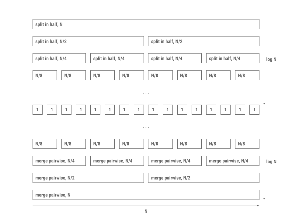
Each level in the diagram is a collection of processes that all together run in linear time. Since there are \(2 \log N\) levels with each level doing work proportional to \(N\), the total time is proportional to \(N \log N\).
To be specific, each level does work proportional to \(N\) because of the merging process,
which happens in a zipper-like fashion. Given two sorted lists, merge should continually
compare the first elements of both lists and interweave the elements into a singular sorted list.
For example, given the lists [2, 6, 7] and [1, 4, 5, 8], merge compares the front of both lists (1 and 2). Because
1 < 2, 1 is moved into the next open spot (in this case, the first position) of the overall sorted list. Note
that 2 does not enter the overall list, because we now must effectively compare [2, 6, 7] with [4, 5, 8] and repeat the process
until there are no more elements that need to be compared and merged.
Merge sort is stable as long as we make sure when merging two halves together that we favor equal elements in the left half.
Now, watch this video on mergeSort before attempting the exercise below!
Exercise: mergeSort #
To test your understanding of merge sort, fill out the mergeSort method in
DLList.java. Be sure to take advantage of the provided merge method - read it through to make sure you understand what it’s doing!
This method should be non-destructive, so the original DLList should not be
modified.
Quicksort #
Another example of dividing and conquering is the quicksort algorithm, which proceeds as follows:
- Split the collection to be sorted into three collections by partitioning around a pivot (or “divider”). One collection consists of elements smaller than the pivot, the second collection consists of elements equal to the pivot, and the third consists of elements greater than or equal to the pivot.
- Recursively call quicksort on each collection.
- Merge the sorted collections by concatenation.
Specifically, this version of quicksort is called “three-way partitioning quicksort” due to the three partitions that the algorithm makes on every call.
Here’s an example of how this might work, sorting an array containing 3, 1, 4, 5, 9, 2, 8, 6.
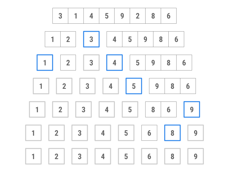
- Choose 3 as the pivot. (We’ll explore how to choose the pivot shortly.)
- Put 4, 5, 9, 8, and 6 into the “large” collection and 1 and 2 into the “small” collection. No elements go in the “equal” collection.
- Sort the large collection into 4, 5, 6, 8, 9; sort the small collection into 1, 2; combine the two collections with the pivot to get 1, 2, 3, 4, 5, 6, 8, 9.
Depending on the implementation, quicksort is not stable because when we move elements to the left and right of our pivot the relative ordering of equal elements can change.
Before moving on to the next part of the lab, check out this video to solidify your understanding of quicksort. Note this was taken from last year’s lecture, so you can stop after the section on quicksort. That is, you can stop at 1:41:00.
Exercise: quicksort #
Some of the code is missing from the quicksort method in DLList.java. Fill
in the function to complete the quicksort implementation.
Be sure to use the supplied helper methods, namely append and addLast! This
method should be non-destructive, so the original DLList should not be
modified.
Discussion: Quicksort #
Discussion 1: Runtime #
First, let’s consider the best-case scenario where each partition divides a range optimally in half. Using some of the strategies picked up from the merge sort analysis, we can determine that quicksort’s best case asymptotic runtime behavior is \(O(N \log N)\). Discuss with your partner why this is the case, and any differences between quicksort’s best case runtime and merge sort’s runtime.
However, quicksort is faster in practice and tends to have better constant factors (which aren’t included in the big-Oh analysis). To see this, let’s examine exactly how quicksort works.
We know concatenation for linked lists can be done in constant time, and for arrays it can be done in linear time. Partitioning can be done in time proportional to the number of elements \(N\). If the partitioning is optimal and splits each range more or less in half, we have a similar logarithmic division of levels downward like in merge sort. On each division, we still do the same linear amount of work as we need to decide whether each element is greater or less than the pivot.
However, once we’ve reached the base case, we don’t need as many steps to reassemble the sorted collection. Remember that with merge sort, while each list of one element is sorted, the entire set of one-element lists is not necessarily in order, which is why there are \(\log N\) steps to merge upwards in merge sort. This isn’t the case with quicksort as each element is in order. Thus, merging in quicksort is simply one level of linear-time concatenation.
Unlike merge sort, quicksort has a worst-case runtime different from its best-case runtime. Suppose we always choose the first element in a range as our pivot. Then, which of the following conditions would cause the worst-case runtime for quicksort? Discuss with your partner, and verify your understanding by highlighting the line below for the answer.
Sorted or Reverse Sorted Array. This is because the pivot will always be an extreme value (the largest or smallest unsorted value) and we will thus have N recursive calls, rather than log(n).
What is the runtime of running quicksort on this array?
Theta(N^2)
Under these conditions, does this special case of quicksort remind you of any other sorting algorithm we’ve discussed in this lab? Discuss with your partner.
We see that quicksort’s worst case scenario is pretty bad… You might be wondering why we’d even bother with it then! However, though it’s outside the scope of this class for you to prove why, we can show that on average, quicksort has \(O(N \log(N))\) runtime! In practice, quicksort ends up being very fast.
Discussion 2: Choosing a Pivot #
Given a random collection of integers, what’s the best possible choice of pivot for quicksort that will break the problem down into \(\log N\) levels? Discuss with your partner and describe an algorithm to find this pivot element. What is its runtime? It’s okay if you think your solution isn’t the most efficient.
Quicksort in Practice #
How fast was the pivot-finding algorithm that you came up with? Finding the exact median of our elements may take so much time that it may not help the overall runtime of quicksort at all. It may be worth it to choose an approximate median, if we can do so really quickly. Options include picking a random element, or picking the median of the first, middle, and last elements. These will at least avoid the worst case we discussed above.
In practice, quicksort turns out to be the fastest of the general-purpose
sorting algorithms we have covered so far. For example, it tends to have better
constant factors than that of merge sort. For this reason, Java uses this
algorithm for sorting arrays of primitive types, such as ints or floats.
With some tuning, the most likely worst-case scenarios are avoided, and the
average case performance is excellent.
Here are some improvements to the quicksort algorithm as implemented in the Java standard library:
- When there are only a few items in a sub-collection (near the base case of the recursion), insertion sort is used instead.
- For larger arrays, more effort is expended on finding a good pivot.
- Various machine-dependent methods are used to optimize the partitioning
algorithm and the
swapoperation. - Dual pivots
For object types, however, Java uses a hybrid of merge sort and insertion sort called “Timsort” instead of quicksort. Can you come up with an explanation as to why? Hint: Think about stability!
Conclusion #
To put together the pieces we saw earlier, watch this video Quicksort versus Mergesort
Summary #
In yesterday’s lab and this lab, we learned about more comparison-based algorithms for sorting collections. Within comparison-based algorithms, we examined two different paradigms for sorting:
- Simple sorts like insertion sort and selection sort which demonstrated algorithms that maintained a sorted section and moved unsorted elements into this sorted section one-by-one. With optimization like heapsort or the right conditions (relatively sorted list in the case of insertion sort), these simple sorts can be fast!
- Divide and conquer sorts like merge sort and quicksort. These algorithms take a different approach to sorting: we instead take advantage of the fact that collections of one element are sorted with respect to themselves. Using recursive procedures, we can break larger sorting problems into smaller subsequences that can be sorted individually and quickly recombined to produce a sorting of the original collection.
Here are several online resources for visualizing sorting algorithms. If you’re having trouble understanding these sorts, use these resources as tools to help build intuition about how each sort works.
- VisuAlgo
- Sorting.at
- Sorting Algorithms Animations
- USF Comparison of Sorting Algorithms
- AlgoRhythmics: sorting demos through folk dance including insertion sort, selection sort, merge sort, and quicksort
To summarize the sorts that we’ve learned, take a look at the following table. If you’d like a refresher on what it means for a sort to be stable or in place, please revisit the lab 20 spec from yesterday:
| Best Case Runtime | Worst Case Runtime | Stable | In Place | Notes | |
|---|---|---|---|---|---|
| Insertion Sort | \(\Theta(N)\) | \(\Theta(N^2)\) | Yes | Yes | |
| Selection Sort | \(\Theta(N^2)\) | \(\Theta(N^2)\) | No | Yes | Can be made stable under certain conditions. |
| Heap Sort | \(\Theta(N \log N)\) | \(\Theta(N \log N)\) | No | Yes | If all elements are equal then runtime is \(\Theta(N)\). Hard to make stable. |
| Merge Sort | \(\Theta(N \log N)\) | \(\Theta(N \log N)\) | Yes | Not usually. Typical implementations are not, and making it in-place is terribly complicated. | An optimized sort called “Timsort” is used by Java for arrays of reference types. |
| Quicksort | \(\Theta(N \log N)\) | \(\Theta(N^2)\) | Depends | Most implementations use log(N) additional space for the recursive stack frames | Stability and runtime depend on partitioning strategy; three-way partition quicksort is stable. If all elements are equal, then the runtime using three-way partition quicksort is \(\Theta(N)\). Used by Java for arrays of primitive types. Fastest in practice. |
You may have noticed that there seems to be a lower bound on how fast our sorting algorithms can go. For comparison based sorts, we can prove the best we can do is \(O(N\log(N))\). You can watch a very brief video explanation here at timestamp 11:42. You can also read a more in-depth proof, if you’re into that kind of thing. Tomorrow, we’ll learn about counting sorts, which can do even better when we’re able to use them.
Deliverables #
To get credit for this lab:
- Complete the following methods in
DLList.java:mergeSortquicksort