
Introduction
There are no new skeleton files for this lab. Instead, create a directory called lab24 in your su18-*** directory and copy your Graph.java file from the last lab into this directory. Then, make a new IntelliJ project.
More Graph Algorithms
Last lab, we introduced graphs and their representations, and then we moved to basic graph iteration. A variety of algorithms for processing graphs are based on this kind of iteration, and we’ve already seen the following algorithms:
- Determining if a path exists between two different vertices
- Finding a path between two different vertices
- Topological sorting
Neither algorithm depended on the representation of the fringe. Either depth-first traversal (using a stack) or breadth-first traversal (using a queue) would have worked.
We’re now going to investigate an algorithm where the ordering of the fringe does matter. But first…
Storing Extra Information
Recall the exercise from last lab where you determined the path from a start vertex to a stop vertex. A solution to this exercise involved building a traversal, and then filtering the vertices that were not on the path. Here was the suggested procedure:
Then, trace back from the finish vertex to the start, by first finding a visited vertex
ufor which(u, finish)is an edge, then a vertexvvisited earlier thanufor which(v, u)is an edge, and so on, finally finding a vertexwfor which(start, w)is an edge (isAdjacentmay be useful here!). Collecting all these vertices in the correct sequence produces the desired path.
Instead of searching for the previous vertex along the path in all of the visited nodes like we did last lab, we can create predecessor links. If each fringe element contains a vertex and its predecessor along the traversed path, we can make the construction of the path more efficient. This is an example where it is useful to store extra information in the fringe along with a vertex.
Associating Distances with Edges
In graph applications we’ve dealt with so far, edges were used only to connect vertices. A given pair of vertices were either connected by an edge or they were not. Other applications, however, process edges with weights, which are numeric values associated with each edge. Remember that in an application, an edge just represents some kind of relationship between two vertices, so the weight of the edge could represent something like the strength, weakness, or cost of that relationship.
In today’s exercises, the weight associated with an edge will represent the distance between the vertices connected by the edge. In other algorithms, a weight might represent the cost of traversing an edge or the time needed to process the edge.
A graph with edge weights is shown below.
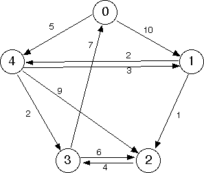
Observe the weights on the edges (the small numbers in the diagram), and note that the weight of an edge (v, w) doesn’t have to be equal to the weight of the edge (w, v), its reverse.
Shortest Paths
A common problem involving a graph with weighted edges is to find the shortest path between two vertices. This means to find the sequence of edges from one vertex to the other such that the sum of weights along the path is smallest.
This is a core problem found in real life mapping applications. Say you want directions from one location to another. Your mapping software will try to find the shortest path from your location (a vertex), to another location (another vertex). Different paths in the graph may have different lengths and different amounts of traffic, which could be the weights of the paths. You would want your software to find the shortest, or fastest, path for you.
Exercise: Shortest Path
Below is the same graph shown previously.
Suppose that the weight of an edge represents the distance along a road between the corresponding vertices. The weight of a path would then be the sum of the weights on its edges.
What is the shortest path that connects vertex 0 with vertex 2? Discuss with your partner, and then submit your answer to the Gradescope assessment. Submit your answer as a space-separated list of numbers.
Dijkstra’s Algorithm
How did you do on the shortest path self-test? It’s pretty tricky, right? Luckily, there is an algorithm devised by Edsger Dijkstra (usually referred to as Dijkstra’s Algorithm), that can find the shortest paths on a graph, and not just for a pair of vertices , but all the shortest paths from a start vertex s to every other vertex reachable from s. The algorithm is somewhat tedious for humans to do by hand, but it isn’t too inefficient for computers.
Below is an overview of the algorithm. The algorithm below finds the shortest paths from a starting vertex to all other nodes in a graph, also known as a shortest paths tree. To just find the shortest path between two specified vertices s and t, simply terminate the algorithm after t has been visited.
- Initialization
-
- Maintain a mapping, from vertices to their distance from the start vertex. This will be used by the fringe to determine the next vertex to visit.
- Add the start vertex to the fringe with distance zero.
- All other nodes can be left out of the fringe. If a node is not in the fringe, assume it has distance infinity.
- For each vertex, keep track of which other node is the predecessor for the node along the shortest path found.
- While Loop
- Loop until the fringe is empty.
-
Let
vbe the vertex in the fringe with the shortest distance to the start. Remove and hold ontov. (One can prove that for this vertex, the shortest path from the start vertex to it is known for sure.) -
If
vis the destination vertex (optional), terminate now. Otherwise, mark it as visited. Any visited vertices should not be visited again. -
Then, for each neighbor
wofv, do the following:-
As an optimization, if
whas been visited already, skip it (as we have no way of finding a shorter path anyways). -
If
wis not in the fringe (or another way to think of it - it’s distance is infinity or undefined in our distance mapping), add it to the fringe (with the appropriate distance and previous pointers). -
Otherwise,
w’s distance might need updating if the path throughvtowis a shorter path than what we’ve seen so far. If that is indeed the case, replace the distance forw’s fringe entry with the distance fromstarttovplus the weight of the edge(v, w), and replace its predecessor withv. If you are using ajava.util.PriorityQueue, you will need to calladdorofferagain so that the priority updates correctly - do not callremoveas this takes linear time.
-
-
Every time a vertex is dequeued from the fringe, that vertex’s shortest path has been found and it is finalized. The algorithm ends when the stop vertex is returned by next. Follow the predecessors to reconstruct the path.
One caveat: although we often use the analogy of finding the shortest path on a map to describe Dijkstra’s algorithm, note that it’s possible to try to run Dijkstra’s on any arbitrary graph structure. This means you may come across a graph with negative edge weights.
For instance, consider a real-life example graph where the vertices are the locations. As a taxi driver, you are paid to drive customers between certain locations. However, you may lose money when you drive to pick up a new customer.
In fact, Dijkstra’s algorithm may not work in general on such graphs with negative edge weights! Consider why this is the case. In CS 170, we’ll learn about the Bellman-Ford algorithm, which solves the same single-source shortest paths problem for graphs with negative edge weights too.
Dijkstra’s Algorithm Animation
Dijkstra’s algorithm is pretty complicated to explain in text, so it might help you to see an animation of it.
As you watch the video, think about the following questions with your partner:
- In the animation you just watched, how can you tell what vertices were currently in the fringe for a given step?
- In the animation you just watched, after the algorithm has been run through, how can you look at the chart and figure out what the shortest path from to is?
Note that in this video, the fringe is initialized by putting all the vertices into it at the beginning with their distance set to infinity. While this is also a valid way to run Dijkstra’s algorithm for finding shortest paths (and one of the original ways it was defined), this is inefficient for large graphs. Semantically, it is the same to think of any vertex not in the fringe as having infinite distance, as a path to it has not yet been found.
Exercise: Dijkstra’s Algorithm
With your partner, run Dijkstra’s algorithm by hand on the pictured graph below, finding the shortest path from vertex 0 to vertex 4. Keep track of what the fringe contains at every step.
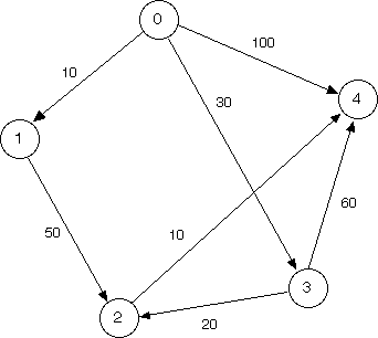
We recommend keeping track of a table like in the animation. Also, please make sure you know what the fringe contains at each step.
Exercise: shortestPath
Add Dijkstra’s algorithm to Graph.java from yesterday. Here’s the method header:
public List<Integer> shortestPath(int start, int stop) {
    // TODO: YOUR CODE HERE
    return null;
}
For this method, you will need to refer to each Edge object’s weight field. Additionally, it may be useful to write a getEdge method, that will return the Edge object corresponding to the input variables. Here’s the header:
public Edge getEdge(int u, int v) {
    // TODO: YOUR CODE HERE
    return null;
}
Hint: At a certain point in Dijkstra’s algorithm, you have to change the value of nodes in the fringe. Java’s PriorityQueue does not support this operation directly, but we can add a new entry into the PriorityQueue that contains the updated value (and will always be dequeued before any previous entries). Then, by tracking which nodes have been visited already, you can simply ignore any copies after the first copy dequeued.
Additionally, adding the vertices to our PriorityQueue fringe directly won’t be enough. Our vertices are integers, so the PriorityQueue will order them by their natural ordering. Write a comparator to change the ordering of the vertices.
Runtime
Implemented properly using a priority queue backed by a binary heap, Dijkstra’s algorithm should run in O((|V| + |E|) log |V|) time. This is because at all times our heap size remains a polynomial factor of |V| (even with lazy removal, our heap size never exceeds |V|^2), and we make at most |V| dequeues and |E| updates requiring heap operations.
For connected graphs, the runtime can be simplified to O(|E| log |V|), as the number of edges must be at least |V| - 1. Using alternative implementations of the priority queue can lead to increased or decreased runtimes.
Bear Maps
With the remaining time in lab, get started on Bear Maps. There will be a project workday on Monday but we encourage you to get started today!
In the project, we’ll be working on implementing a similar shortest paths algorithm that runs on a weighted, undirected graph of the city of Berkeley. One advantage of working with a map that represents real distances in the world is that we can take advantage of information about the world like the straightline distance between two points and use that as a heuristic to help guide our search process.
Recall that Dijkstra’s algorithm can help us solve the single-source shortest paths problem by computing the shortest paths tree from a source vertex, s, all other vertices in the graph. We might think of Dijkstra’s algorithm as similar to breadth-first search on unweighted graphs since it’s just trying to expand its fringe outwards by picking the nearest vertices first, without any regard for moving in particular direction.
But if we only care about going from one start vertex to one end vertex, we can use a distance heuristic to point the search algorithm in the direction of the goal. This smaller problem of finding the shortest path between a pair of points is called single-pair shortest paths, and in the project, we’ll implement the A* Search algorithm to speed up the computation for this shortest path.
Optional Applications
Graphs have very real applications! In Bear Maps, we use a graph to represent data about the real world. We can also use graphs to solve other problems in computer science such as:
- Garbage Collection, the problem of managing memory in Java.
- Search engines utilize algorithms (most famously, Google’s PageRank) to sovle the problem of organizing information on the internet and making efficient queries on the data to return the best results.
Deliverables
- Complete the
shortestPathmethod inGraph.java. - Complete the self-reflection linked in the Gradescope assessment.