
Before You Begin
You should continue working with your project 1 partner for today’s lab, out of your
su19-proj1-s***-s***repository.
Pull the files for lab 7 from the skeleton.
Learning Goals
“An engineer will do for a dime what any fool will do for a dollar. — Arthur M. Wellington”
—Paul Hilfinger
Efficiency comes in two flavors:
- Programming cost
-
- How long does it take to develop your programs?
- How easy is it to read or modify your code?
- How maintainable is your code?
- Execution cost
-
- Time complexity: How much time does your program take to execute?
- Space complexity: How much memory does your program require?
We’ve already seen many examples of reducing programming cost. We’ve written unit tests and employed test-driven development to spend a little more time up front writing tests to save a lot of time down the line debugging programs. And we’ve seen how encapsulation can help reduce the cognitive load that a programmer needs to deal with by allowing them to think in terms of high-level abstractions like lists instead of having to deal with the nitty-gritty details of pointer manipulation.
We’ve only just scratched the surface on methods for reducing and optimizing programming costs, but for the coming weeks, it’ll be helpful to have a working understanding of the idea of execution cost.
In this lab, we consider ways of measuring the efficiency of a given code segment. Given a function f, we want to find out how fast that function runs.
Algorithms
An algorithm is a step-by-step procedure for solving a problem, or an abstract notion that describes an approach for solving a problem. The code we write in this class, our programs, are implementations of algorithms. Indeed, we’ve already written many algorithms: the methods we’ve written for IntList, SLList, LinkedListDeque, and ArrayDeque are all algorithms that operate on data by storing and accessing that data in different ways.
As another example, consider the problem of sorting a list of numbers. One algorithm we might use to solve this problem is called bubble sort. Bubble sort tells us we can sort a list by repeatedly looping through the list and swapping adjacent items if they are out of order, until the entire sorting is complete.
Another algorithm we might use to solve this problem is called insertion sort. Insertion sort says to sort a list by looping through our list, taking out each item we find, and putting it into a new list in the correct order.
Several websites like VisuAlgo, Sorting.at, Sorting Algorithms, and USF have developed some animations that can help us visualize these sorting algorithms. Spend a little time playing around with these demos to get an understanding of how much time it takes for bubble sort or insertion sort to completely sort a list. We’ll revisit sorting in more detail later in this course, but for now, try to get a feeling of how long each algorithm takes to sort a list. How many comparison does each sort need? And how many swaps?
Since each comparison and each swap takes time, we want to know which is the faster algorithm: bubble sort or insertion sort? And how fast can we make our Java programs that implement them? Much of our subsequent work in this course will involve estimating program efficiency and differentiating between fast algorithms and slow algorithms. This set of activities introduces an approach to making these estimates.
Measuring Execution Time
One way to estimate the time an algorithm takes is to measure the time it takes to run the program directly. Each computer has an internal clock that keeps track of time, usually in the number of fractions of a second that have elapsed since a given base date. The Java method that accesses the clock is System.currentTimeMillis. A Timer class is provided in Timer.java.
Take some time now to find out exactly what value System.currentTimeMillis returns, and how to use the Timer class to measure the time taken by a given segment of code.
Exercise: Sorter
The file Sorter.java contains a version of the insertion sort algorithm mentioned earlier. Its main method uses a command-line argument to determine how many items to sort. It fills an array of the specified size with randomly generated values, starts a timer, sorts the array, and prints the elapsed time when the sorting is finished.
javac Sorter.java
java Sorter 300
Compiling and running Sorter like above will tell us exactly how long it takes to sort an array of 300 randomly chosen elements.
Copy Sorter.java to your directory, compile it, and then determine the size of the smallest array that needs 1 second (1000 milliseconds) to sort. An answer within 100 elements is fine.
How fast is Sorter.java? What’s the smallest array size that you and your partner found that takes at least 1 second to sort?
You may notice that your partner will end up with different timing results and a different number of elements.
Worksheet: 1. Timing
Complete this exercise on your worksheet.
Counting Steps
From timing the program in the previous example, we learned it isn’t very helpful in determining how good an algorithm is; different computers end up with different results! An alternative approach is step counting. The number of times a given step, or instruction, in a program gets executed is independent of the computer on which the program is run and is similar for programs coded in related languages. With step counting, we can now formally and deterministically describe the runtime of programs.
We define a single step as the execution of a single instruction or primitive function call. For example, the + operator which adds two numbers is considered a single step. We can see that 1 + 2 + 3 can be broken down into two steps where the first is 1 + 2 while the second takes that result and adds it to 3. From here, we can combine simple steps into larger and more complex expressions.
(3 + 3 * 8) % 3
This expression takes 3 steps to complete: one for multiplication, one for addition, and one for the modulus of the result.
From expressions, we can construct statements. An assignment statement, for instance, combines an expression with one more step to assign the result of the expression to a variable.
int a = 4 * 6;
int b = 9 * (a - 24) / (9 - 7);
In the example above, each assignment statement takes one additional step on top of however many steps it took to compute the right-hand side expressions. In this case, the first assignment to a takes one step to compute 4 * 6 and one more step to assign the result, 24, to the variable a. How many steps does it take to finish the assignment to b?
Here are some rules about what we count as taking a single step to compute:
- Assignment and variable declaration statements
- All unary (like negation) and binary (like addition/and/or) operators
- Function calls
returnstatements
One important case to be aware of is that, while calling a function takes a single step to setup, executing the body of the function may require us to do much more than a single step of work.
Counting Conditionals
With conditional statements like if statements, the total step count depends on the outcome of the condition we are testing.
if (a > b) {
    temp = a;
    a = b;
    b = temp;
}
The example above can take four steps to execute: one for evaluating the conditional expression a > b and three steps for evaluating each line in the body of the condition. But this is only the case if a > b. If the condition is not true, then it only takes one step to check the conditional expression.
That leads us to consider two quantities: the worst case count, or the maximum number of steps a program can execute, and the best case count, or the minimum number of steps a program needs to execute. The worst case count for the program segment above is 4 and the best case count is 1.
Worksheet: 2. Counting
Complete this exercise on your worksheet.
Loop Counting
for (int k = 0; k < N; k++) {
    sum = sum + 1;
}
In terms of \(N\), how many operations are executed in this loop? Remember that each of the actions in the for-loop header (the initialization of k, the exit condition, and the increment) count too!
It takes 1 step to execute the initialization,
int k = 0. Then, to execute the loop, we have the following sequence of steps:
- Check the loop condition,
k < N- Add 1 to the
sum- Update the value of
sumby assignment- Increment the loop counter,
k- Update
kby assignmentThis accounts for the first \(1 + 5N\) steps. In the very last iteration of the loop, after we increment
ksuch thatknow equals \(N\), we spend one more step checking the loop condition again to figure out that we need to finally exit the loop so the final number of steps is \(1 + 5N + 1\).
Now consider code for the remove method which removes the item at a given position of an array values by shifting over all the remaining elements.
void remove(int pos) {
    for (int k = pos + 1; k < len; k++) {
        values[k - 1] = values[k];
    }
    len -= 1;
}
The counts here depend on pos. Each column in the table below shows the total number of steps for computing each value of pos.
| category | pos = 0 | pos = 1 | pos = 2 | … | pos = len - 1 |
|---|---|---|---|---|---|
pos + 1 | 1 | 1 | 1 | 1 | |
assignment to k | 1 | 1 | 1 | 1 | |
| loop conditional | len | len - 1 | len - 2 | 1 | |
increment to k | len - 1 | len - 2 | len - 3 | 0 | |
update k | len - 1 | len - 2 | len - 3 | 0 | |
| array access | len - 1 | len - 2 | len - 3 | 0 | |
| array assignment | len - 1 | len - 2 | len - 3 | 0 | |
decrement to len | 1 | 1 | 1 | 1 | |
assignment to len | 1 | 1 | 1 | 1 | |
| Total count | 5 * len | 5 * len - 4 | 5 * len - 8 | 5 |
We can summarize these results as follows: a call to remove with argument pos requires in total:
- 1 step to calculate
pos + 1 - 1 step to make the initial assignment to
k len - posloop testslen - pos - 1increments ofklen - pos - 1reassignments toklen - pos - 1accesses tovalueselementslen - pos - 1assignments tovalueselements- 1 step to decrement
len - 1 step to reassign to
len
If all these operations take roughly the same amount of time, the total is 5 * (len - pos). Notice how we write the number of statements as a function of the input argument. For a small value of pos, the number of steps executed will be greater than if we had a larger value of pos. And vice versa: a larger value of pos will reduce the number of steps we need to execute.
Counting steps in nested loops is a little more involved. As an example, we’ll consider an implementation of the method removeZeroes.
void removeZeroes() {
    int k = 0;
    while (k < len) {
        if (values[k] == 0) {
            remove(k);
        } else {
            k += 1;
        }
    }
}
Intuitively, the code should be slowest on an input where we need to do the most work, or an array of values full of zeroes. Here, we can tell that there is a worst case—removing everything—and a best case, removing nothing. To calculate the runtime, like before, we start by creating a table to help organize information.
| category | best case | worst case |
|---|---|---|
assignment to k | 1 | 1 |
| loop conditional | len + 1 | len + 1 |
| array accesses | len | len |
| comparisons | len | len |
| calls to remove | 0 | len |
| k + 1 | len | 0 |
update to k | len | 0 |
In the best case, we never call remove so its runtime is simply the sum of the rows in the “best case” column. Thus, the best-case count is 1 + 5 * len + 1.
The only thing left to analyze is the worst-case scenario. Remember that the worst case makes len total calls to remove. We already approximated the cost of a call to remove for a given pos and len value earlier: 5 * (len - pos).
In our removals, pos is always 0, and only len is changing. The total cost of the removals is shown below.
The challenge now is to simplify the expression. A handy summation formula to remember is the sum of the first \(k\) natural numbers.
\[1 + 2 + \cdots + k = \frac{k(k + 1)}{2}\]This lets us simplify the cost of removals. Remembering to include the additional steps in the table, we can now express the worst-case count of removeZeroes as:
We often prefer to simplify this by substituting len for a symbolic name like \(N\).
That took… a while.
Abbreviated Estimates
From this section onwards, we present a set of fairly precise definitions, and we’ll be relying on the example developed in this part and the previous part to help us build a solid definition for asymptotic notation. If you’re not fully comfortable with any of the material so far, now is the perfect time to review it with your partner, an academic intern, or a staff member.
Producing step count figures for even those simple program segments took a lot of work. But normally we don’t actually need an exact step count but rather just an estimate of how many steps will be executed.
In most cases, we only care about what happens for very large \(N\) as that’s where the differences between algorithms and their execution time really become limiting factors in the scalability of a program. We want to consider what types of algorithms would best handle big amounts of data, such as in the examples listed below:
- Simulation of billions of interacting particles
- Social network with billions of users
- Encoding billions of bytes of video data
The asymptotic behavior of a function f (any one of the programs above, for example) is a description of how the execution time of f changes as the value of \(N\) grows increasingly large towards infinity. Our goal is to come up with a technique that can be used to compare and contrast two algorithms to identify which algorithm scales better for large values of \(N\).
We can then compute the order of growth of a program, a classification of how the execution time of the program changes as the size of the input grows larger and larger.
We say that the order of growth of \(2N + 3\) is \(N\) since, for large values of \(N\), \(2N + 3\) will be less than \(3N\) and slightly greater than \(2N\). As \(N\) tends towards infinity, the \(+ 3\) contributes less and less to the overall runtime.
This pattern holds for higher-order terms too. Applying this estimation technique to the removeZeroes method above results in the following orders of growth.
- The order of growth for the best-case runtime of
removeZeroes, \(5N + 2\), is proportional to the length of the array, \(N\). - The order of growth for the worst-case runtime of
removeZeroes, \(5 \frac{N(N + 1)}{2} + 3N + 2\), is \(N^2\).
The intuitive simplification being made here is that we discard all but the most significant term of the estimate and also any constant factor of that term. Later, we will see exactly why this is true with a more formal proof.
Asymptotic Analysis
Recap: Simplified Analysis Process
Rather than building the entire table of all the exact step counts, we can instead follow a simplified analysis process.
- Choose a cost model
- These are the underlying assumptions about the costs of each step or instruction for our machine. In this course, we’ll assume all of the basic operations (Java operators, assignment statements,
returnstatements, array access) each take the same, 1 unit of time, but in CS 61C, we’ll see how this fundamental assumption often isn’t true. - Compute the order of growth
- Given the cost model, we can then compute the order of growth for a program. In the
removeZeroesexample, we saw how we could compute an exact count and then find the correct order of growth runtime classification for it by simplifying the expression.
Later, we’ll learn a few shortcuts and practice building intuition/inspection to determine orders of growth, but it’s helpful to remember that we’re always solving the same fundamental problem of measuring how long it takes to run a program, and how that runtime changes as we increase the value of \(N\).
Big-Theta Notation
Computer scientists often use special notation to describe runtime. The first one we’ll learn is called big-theta, represented by the symbol \(\Theta\).
Suppose we have a function, \(f(N)\), with order of growth \(g(N)\). We could say,
\(f(N) \in \Theta(g(N))\), or “\(f(N)\) is in \(\Theta(g(N))\)”
Why do we say “in” \(\Theta\)? Formally, \(\Theta(g(N))\) is a family of functions that all grow proportional to \(f\). Thinking back to our working definition of order of growth as a method for classification, \(\Theta(g(N))\) refers to the entire set of all functions that share the same order of growth.
The advantage of using notation like big-theta is that it provides a common definition for asymptotic analysis which reduces the amount of explaining we need to do when we want to share our ideas with others. It also makes sure we’re all on the same page with the claims we make, so long as we use them carefully and precisely.
Learning new notation can be a little daunting, but we’ve actually already been making statements in big-theta terms. The first claim about removeZeroes that we made earlier,
The order of growth for the best-case runtime of
removeZeroes, \(5N + 2\), is proportional to the length of the array, \(N\).
is essentially equivalent to the claim: In the best-case, removeZeroes is in \(\Theta(N)\).
And, likewise, the second claim that we made earlier,
The order of growth for the worst-case runtime of
removeZeroes, \(5 \frac{N(N + 1)}{2} + 3N + 2\), is \(N^2\).
has its own equivalent in big-theta notation: In the worst-case, removeZeroes is in \(\Theta(N^2)\).
When we use
removeZeroeshere, we mean the runtime of the function rather than the function itself. In practice, we’ll often use this English shortcut as long as the meaning is clearly communicated, though it would be more accurate to say the runtime of the function.
Be Sure to Define N
You may have observed, in our analysis of removeZeroes, that we were careful to make clear what the running time estimate depended on, namely the value of len and the position of the removal.
Unfortunately, students are sometimes careless about specifying the quantity on which an estimate depends. Don’t just use \(N\) without making clear what \(N\) means. This distinction is important especially when we begin to touch on sorting later in the course. It may not always be clear what \(N\) means.
We’ll often qualify our runtimes by stating, “where \(N\) is the length of the list”, but we often also say things like, “where \(N\) is the value of the largest number in the list”.
Formal Definitions
Big-Theta
Formally, we say that \(f(N) \in \Theta(g(N))\) if and only if there exist positive constants \(k_1, k_2\) such that \(k_1 g(N) \leq f(N) \leq k_2 g(N)\) for all \(N\) greater than some \(N_0\) (very large \(N\)).
In other words, \(f(N)\) must be bounded above and below by \(g(N)\) asymptotically. But we’ve already seen something like this too.
We say that the order of growth of \(2N + 3\) is \(N\) since, for large values of \(N\), \(2N + 3\) will be less than \(3N\) and slightly greater than \(2N\). As \(N\) tends towards infinity, the \(+ 3\) contributes less and less to the overall runtime.
In this example, we chose \(k_1 = 2\) and \(k_2 = 3\). These two choices of \(k\) constitute a tight-bound for \(2N + 3\) for all values of \(N \geq 3\).
This idea of big-theta notation as a tight-bound is very useful as it allows us to, very precisely, state exactly how scalable a function’s runtime grows as the size of its input (\(N\)) grows. When a \(\Theta(N)\) function’s input size increases, we’d expect the runtime to also increase linearly.
Translating the first paragraph of this section word-for-word to mathematical language, we have:
Big-Theta Definition 1
We say that
\[f(N) \in \Theta(g(N))\]iff \(\quad \exists\) \(k_1, k_2 > 0 \quad\) s.t. \(\quad k_1 g(N) \leq f(N) \leq k_2 g(N) \quad\) \(\forall\) \(N > N_0\).
There is also an alternate formal definition of Big-Theta which is equivalent.
Big-Theta Definition 2
\[f(N) \in \Theta(g(N)) \implies \lim_{N \rightarrow \infty} \frac{f(N)}{g(N)} = c\]where
.
Notice how this definition similarly enforces large inputs \(N\), via the fact that it takes the limit as \(N\) becomes infinitely large. Also notice how \(f(N)\) and \(g(N)\) differs from each other by only a factor of \(c\). Since this condition means that \(f\) and \(g\) are of the same magnitude, it is clear that given this we would always be able to introduce constant scalars to satisfy the constraint involving \(k_1\) and \(k_2\) in the first definition.
Taking a look at our example from before, we see that this definition confirms again that \(2N + 3 \in \Theta(N)\), since \(\lim_{N \rightarrow \infty} \frac{2N+3}{N} = 2\), and \(2\) is a constant between \(0\) and \(\infty\).
Big-O
But, there are many scenarios where we can’t actually give a tight bound: sometimes, it just doesn’t exist. And, practically-speaking, one of the common use scenarios for runtime in the real world is to help choose between several different algorithms with different orders of growth. For these purposes, it’s often sufficient just to give an upper-bound on the runtime of a program.
There exists a very common asymptotic notation, big-O, represented by the symbol, \(O\).
Likewise, the formal definition for big-O follows, \(f(N) \in O(g(N))\) if and only if there exists a positive constant \(k_2\) such that \(f(N) \leq k_2 g(N)\) for all \(N\) greater than some \(N_0\) (very large \(N\)).
Big-O Definition 1
We say that
\[f(N) \in O(g(N))\]iff \(\quad \exists\) \(k_2 > 0 \quad\) s.t. \(\quad f(N) \leq k_2 g(N) \quad\) \(\forall\) \(N > N_0\).
Note that this is a looser condition than big-theta since big-O doesn’t include the lower bound.
The limit definition is as follows:
Big-O Definition 2
\[f(N) \in O(g(N)) \implies \lim_{N \rightarrow \infty} \frac{f(N)}{g(N)} \text{ \textless } \infty\]
Big-Omega
Similarly, we can also give a lower-bound on the runtime of a program. This asymptotic notation, big-Omega, is represented by the symbol, \(\Omega\).
Likewise, the formal definition for big-Omega follows, \(f(N) \in \Omega(g(N))\) if and only if there exists a positive constant \(k_1\) such that \(f(N) \geq k_1 g(N)\) for all \(N\) greater than some \(N_0\) (very large \(N\)).
Big-Omega Definition
We say that
\[f(N) \in \Omega(g(N))\]iff \(\quad \exists\) \(k_1 > 0 \quad\) s.t. \(\quad f(N) \geq k_1 g(N) \quad\) \(\forall\) \(N > N_0\).
Note that this is a looser condition than big-theta since big-Omega doesn’t include the upper bound.
The limit definition is as follows:
Big-Omega Definition 2
\[f(N) \in \Omega(g(N)) \implies \lim_{N \rightarrow \infty} \frac{f(N)}{g(N)} > 0\]
Math Tips and Tricks
Common Orders of Growth
Here are some commonly-occurring estimates listed from no growth at all to fastest growth.
- Constant time, often indicated with \(1\).
- Logarithmic time or proportional to \(\log N\).
- Linear time or proportional to \(N\).
- Linearithmic time or proportional to \(N \log N\).
- Quadratic/polynomial time or proportional to \(N^{2}\).
- Exponential time or proportional to \(k^{N}\) for some constant \(k\).
- Factorial time or proportional to \(N!\) (\(N\) factorial).
L’Hopital’s Rule
If absolutely necessary, we can apply L’Hopital’s rule to help us solve the limit if we are using our second defintion of these asymptotic bounds. It tells us that in the case of indeterminate forms, we have that:
\[\lim_{N \rightarrow \infty} {f(N) \over g(N)} = \lim_{N \rightarrow \infty} {f'(N) \over g'(N)}\]Hopefully you will soon build the intuition to avoid having to do this, but just to show that it will work, here’s an example:
Question: Given \(f(N) = N^{5}\) and \(g(N) = 5^{N}\), is \(f(N) \text{ in } \Theta(g(N))\)?
Solution: After repeatedly applying L’hopital’s rule, we see that \(f(N) \text{ is not in } \Theta(g(N))\):
\[\lim\limits_{N \to \infty} \frac{f(N)}{g(N)} = \lim\limits_{N \to \infty} \frac{N^{5}}{5^{N}} = \lim\limits_{N \to \infty} \frac{5N^{4}}{5^{N} \log 5} = \cdots = \lim\limits_{N \to \infty} \frac{5!}{5^{N} \log^5 5} = 0\]This tells us that actually here, \(f(N) \in O(g(N))\)
Note that this holds consistent with our Common Orders of Growth list above; it is always true that exponential factors grow much faster than any polynomial.
Logarithmic Algorithms
We will shortly encounter algorithms that run in time proportional to \(\log N\) for some suitably defined \(N\). Recall from algebra that the base-10 logarithm of a value is the exponent to which 10 must be raised to produce the value. It is usually abbreviated as \(\log_{10}\). Thus
- \(\log_{10} 1000\) is 3 because \(10^{3} = 1000\).
- \(\log_{10} 90\) is slightly less than 2 because \(10^{2} = 100\).
- \(\log_{10} 1\) is 0 because \(10^{0} = 1\).
In algorithms, we commonly deal with the base-2 logarithm, written as \(\lg\), defined similarly.
- \(\lg 1024\) is 10 because \(2^{10} = 1024\).
- \(\lg 9\) is slightly more than 3 because \(2^{3} = 8\).
- \(\lg 1\) is 0 because \(2^{0} = 1\).
Another way to think of log is the following: \(\log_{\text{base}} N\) is the number of times \(N\) must be divided by the base before it hits 1. For the purposes of determining orders of growth, however, the log base actually doesn’t make a difference because, by the change of base formula, we know that any logarithm of \(N\) is within a constant factor of any other logarithm of \(N\). We usually express a logarithmic algorithm as simply \(\log N\) as a result.
- Change of Base Formula
- \[\log_b x = \frac{\log_a x}{\log_a b}\]
Algorithms for which the running time is logarithmic are those where processing discards a large proportion of values in each iterations. The binary search algorithm is an example. We can use binary search in order to guess a number that a person in thinking. In each iteration, the algorithm discards half the possible values for the searched-for number, repeatedly dividing the size of the problem by 2 until there is only one value left.
For example, say you started with a range of 1024 numbers in the number guessing game. Each time you would discard half of the numbers so that each round would have the following numbers under consideration:
| Round # | Numbers left |
|---|---|
| 1 | 1024 |
| 2 | 512 |
| 3 | 256 |
| 4 | 128 |
| 5 | 64 |
| 6 | 32 |
| 7 | 16 |
| 8 | 8 |
| 9 | 4 |
| 10 | 2 |
| 11 | 1 |
We know from above that \(\lg 1024 = 10\) which gives us an approximation of how many rounds it will take. We will see further applications of logarithmic behavior when we work with trees in subsequent activities.
Common Summations
These two summations are often useful to us. You can remember them by simply remembering these geometric derivations.
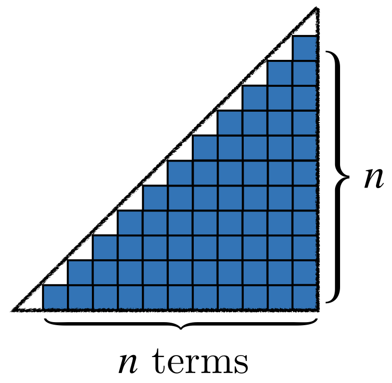
\(1 + 2 + 3 + 4 + \cdots + N\) is in \(\Theta(N^2)\).
Lining up stacks of unit squares, each equal to the number of a corresponding term in the summation, we see that we have a rough triangle, that is almost half of a giant square with side lengths of \(N\). We know that the area of a triangle is half base times height, and so we have that the area of our unit squares is roughly \({1\over2}N^2\), which is in \(\Theta(N^2)\).
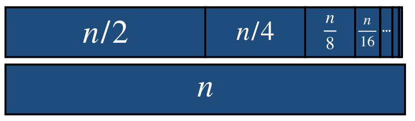
\(1 + 2 + 4 + 8 + \cdots + N\) is in \(\Theta(N)\).
Again, representing each term with unit squares, we see that we can arrange all of the squares to make almost 2 whole bars of length \(N\) (since each term is half as big as the one after it), and \(2N \in \Theta(N)\).
Analyzing Iteration
We’ve thus far defined the language of asymptotic analysis and developed some simple methods based on counting the total number of steps. However, the kind of problems we want to solve are often too complex to think of just in terms of number iterations times however much work is done per iteration.
Consider the following function, repeatedSum.
long repeatedSum(int[] values) {
    int N = values.length;
    long sum = 0;
    for (int i = 0; i < N; i += 1) {
        for (int j = i; j < N; j += 1) {
            sum += values[j];
        }
    }
    return sum;
}
In repeatedSum, we’re given an array of values of length N. We want to take the repeated sum over the array as defined by the following sequence of j’s.
Notice that each time, the number of elements, or the iterations of j, being added is reduced by 1. While in the first iteration, we sum over all \(N\) elements, in the second iteration, we only sum over \(N - 1\) elements. On the next iteration, even fewer: just \(N - 2\) elements. This pattern continues until the outer loop, i, has incremented all the way to \(N\).
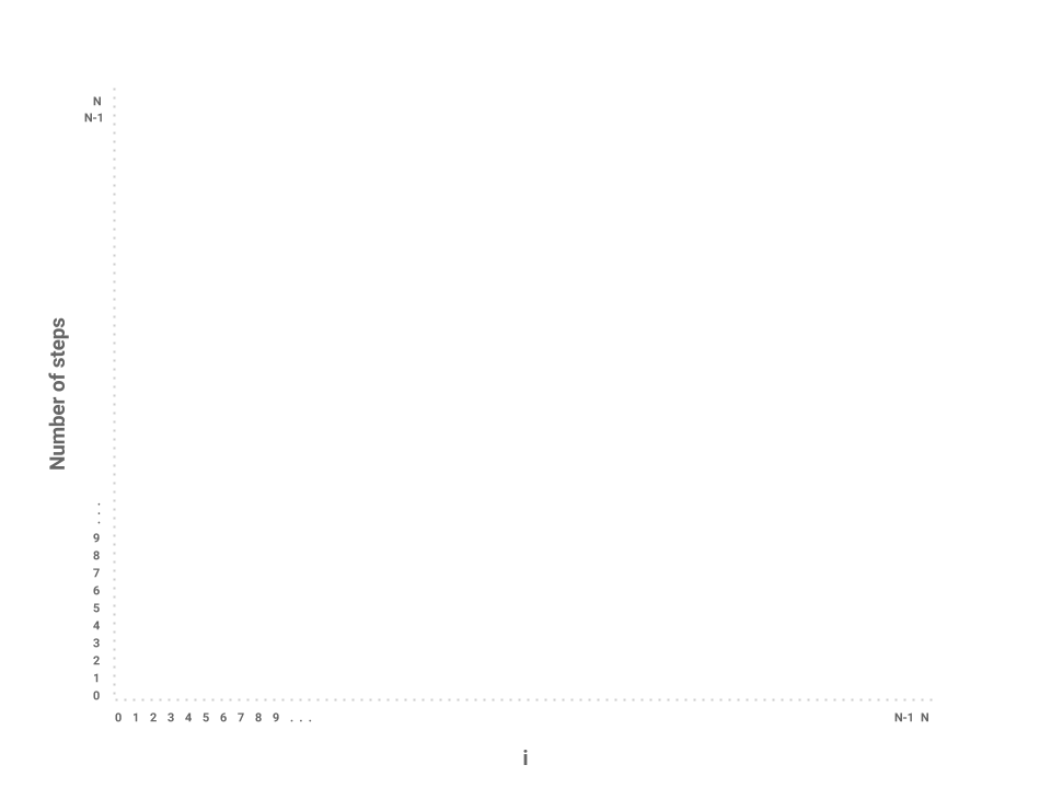
One possible approach to this problem is to draw a bar chart to visualize how much work is being done for each iteration of i. We can represent this by plotting the values of i across the X-axis of the chart and the number of steps for each corresponding value of i across the Y-axis of the chart.
Now, let’s plot the amount of work being done on the first iteration of i where i = 0. If we examine this iteration alone, we just need to measure the amount of work done by the j loop. In this case, the j loop does work proportional to \(N\) steps as the loop starts at 0, increments by 1, and only terminates when j = N.
How about the next iteration of i? The loop starts at 1 now instead of 0 but still terminates at \(N\). In this case, the j loop is proportional to \(N - 1\) steps. The next loop, then, is proportional to \(N - 2\) steps.
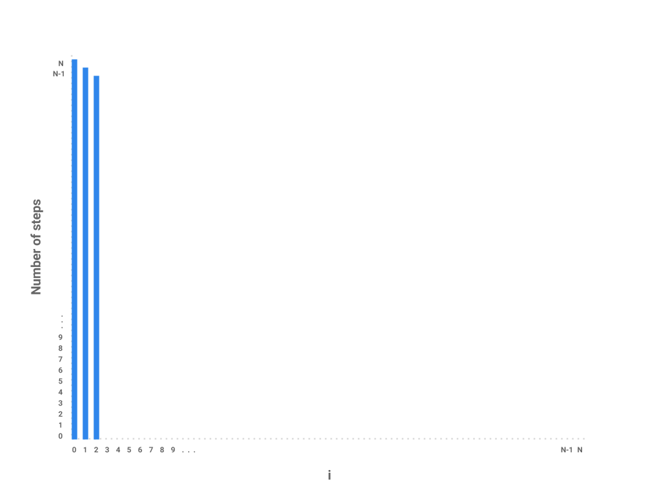
We can start to see a pattern forming. As i increases by 1, the amount of work done on each corresponding j loop decreases by 1. As i approaches \(N\), the number of steps in the j loop approaches 0. In the final iteration, when i = N - 1, the j loop performs work proportional to 1 step.
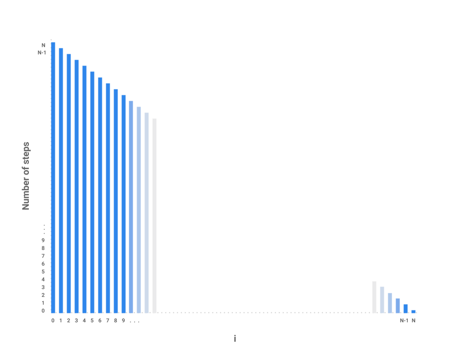
We’ve now roughly measured each loop proportional to some number of steps. Each independent bar represents the amount of work any one iteration of i will perform. The runtime of the entire function repeatedSum then is the sum of all the bars, or simply the area underneath the line.
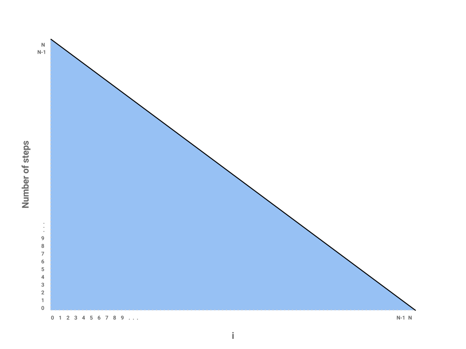
The problem is now reduced to finding the area of a triangle with a base of \(N\) and height of also \(N\). Thus, the runtime of repeatedSum is in \(\Theta(N^{2})\).
We can verify this result mathematically by noticing that the sequence can be described by the following summation:
\(1 + 2 + 3 + ... + N = \frac{N(N + 1)}{2}\) or, roughly, \(\frac{N^{2}}{2}\) which is in \(\Theta(N^{2})\). Hey look! It’s one of our common summations from the above section!
Analyzing Recursion
Now that we’ve learned how to use a bar chart to represent the runtime of an iterative function, let’s try the technique out on a recursive function, mitosis.
int mitosis(int N) {
    if (N == 1) {
        return 1;
    }
    return mitosis(N / 2) + mitosis(N / 2);
}
Let’s start by trying to map each \(N\) over the x-axis like we did before and try to see how much work is done for each call to the function. The conditional contributes a constant amount of work to each call. But notice that in our return statement, we make two recursive calls to mitosis. How do we represent the runtime for these calls? We know that each call to mitosis does a constant amount of work evaluating the conditional base case but it’s much more difficult to model exactly how much work each recursive call will do. While a bar chart is a very useful way of representing the runtime of iterative functions, it’s not always the right tool for recursive functions.
Instead, let’s try another strategy: drawing call trees. Like the charting approach we used for iteration earlier, the call tree will reduce the complexity of the problem and allow us to find the overall runtime of the program on large values of \(N\) by taking the tree recursion out of the problem. Consider the call tree for fib below.
int fib(int N) {
    if (N <= 1) {
        return 1;
    }
    return fib(n - 1) + fib(n - 2);
}
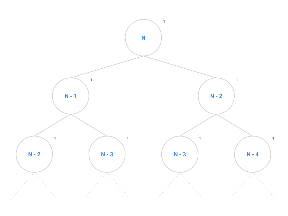
At the root of the tree, we make our first call to fib(n). The recursive calls to fib(n - 1) and fib(n - 2) are modeled as the two children of the root node. We say that this tree has a branching factor of two as each node contains two children. It takes a constant number of instructions to evaluate the conditional, addition operator, and the return statement as denoted by the 1.
We can see this pattern occurs for all nodes in the tree: each node performs the same constant number of operations if we don’t consider recursive calls. If we can come up with a scheme to count all the nodes, then we can simply multiply by the constant number of operations to find the overall runtime of fib.
Remember that the number of nodes in a tree is calculated as the branching factor, \(b\), raised to the height of the tree, \(h\), or \(b^{h}\). Spend a little time thinking about the maximum height of this tree: when does the base case tell us the tree recursion will stop?
Returning to the original problem of mitosis, the call tree is setup just like fib except instead of decrementing \(N\) by 1 or 2, we now divide \(N\) in half each time. Each node performs a constant amount of work but also makes two recursive calls to mitosis(N / 2).
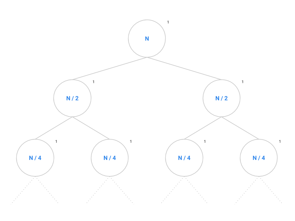
Like before, we want to identify both the branching factor and the height of the tree. In this case, the branching factor is 2 like before. Recall that the series \(N, N/2, \cdots , 4, 2, 1\) contains \(\log_{2} N\) elements since, if we start at \(N\) and break the problem down in half each time, it will take us approximately \(\log_{2} N\) steps to completely reduce down to 1.
Plugging into the formula, we get \(2^{\log_{2} N}\) nodes which simplifies to \(N\). Therefore, \(N\) nodes performing a constant amount of work each will give us an overall runtime in \(\Theta(N)\).
In general, for a recursion tree, we can think of the total work as \(\sum_{\text{layers}} \frac{\text{nodes}}{\text{layer} }\frac{\text{work}}{\text{node}}\) For mitosis, we have \(\lg N\) layers, \(2^i\) nodes in layer \(i\), with \(1\) work per node. Thus we see the sumation \(\sum_{i = 0}^{\lg N} 2^i (1)\), which is exactly the quantity we just calculated.
Best Case and Worst Case
Matt’s friend Caitlyn regularly picks up Gabe after school. One day, Gabe told Caitlyn that he was hungry, and so she took him to grab an after-school snack. They decided on a nearby restaurant that seemed affordable. But although the waiter handed Gabe a kid’s menu, Gabe didn’t want a $4 grilled cheese. Nope, he insisted on getting a $25 steak from the adult’s menu instead! Of course, you can guess how this must have ended–they got the steak. Now when the bill came, how much did they pay? Exactly $25 (plus tax and a nice tip).
Notice that they were not given the option to pay $25 or less, they were to pay exactly $25 in this worst case scenario.
Now before they went in to the restaurant, the question at hand was different. The question was “what is the price range of this restaurant?”. Going into the restaurant, you can expect to pay at least $4 and no more than $25. It is a range.
When answering questions related to asymptotics, the bound you use for your answer depends on the question being asked.
- If you are asked for the runtime, give a single Big Theta bound if possible, or if it is impossible to bound it by a single order of growth, then describe it by providing a Big O for the upper bound and a Big Omega for the lower bound. (Just like how we described the price range of the restaurant.)
- If you are asked for the best and worst case, then give a single Big Theta bound to describe the best case scenario (if possible), and give a single Big Theta bound to describe the worst case scenario (if possible). (Just like how if you ordered the grilled cheese, you would pay exactly $4, and if you ordered the steak, you would pay exactly $25.)
Big Omega is not the same as Best Case and Big O is not the same as Worst Case.
Worksheet: 3. Using the Right Bounds
Complete this exercise on your worksheet.
Practical Tips
- Before attempting to calculate a function’s runtime, first try to understand what the function does.
- Try some small sample inputs to get a better intuition of what the function’s runtime is like. What is the function doing with the input? How does the runtime change as the input size increases? Can you spot any ‘gotchas’ in the code that might invalidate our findings for larger inputs? Remember, the small inputs are just to help you get a feel for what the algorithm does, when we give our runtime though, we only care about large inputs (and thus no, the best case is not \(\Theta(1)\) just because there is a base case).
- Determine if it will be necessary to separate your analysis into a best case answer and a worst case answer.
- If the function is recursive, draw a call tree to map out the recursive calls. This breaks the problem down into smaller parts that we can analyze individually. Once each part of the tree has been analyzed, we can then reassemble all the parts to determine the overall runtime of the function.
- If the function has a complicated loop, draw a bar chart to map out how much work the body of the loop executes for each iteration.
Worksheet: 4. Analyzing Functions
Complete this exercise on your worksheet.
Recap
Our goal today was to figure out how to quantitatively say whether one algorithm is faster than another. We first tried timing the number of seconds programs took to run, but it seemed impractical due to how much our results fluctuated. We then tried to choose a cost model and count the number of operations in the code. This was better since we didn’t have to run the program anymore, but this was a very tedious process. Ultimately, we settled upon asymptotic analysis, in which we estimate the order of growth instead.
We learned about Big-Theta, Big-O, and Big-Omega, which represent a tight bound, upper bound, and lower bound, respectively. We were given two definitions for each of these. Intuitively, we don’t care about lower order terms, and we don’t care about constant scalar multipliers, since these are all insignificant for large inputs \(N\).
We saw examples of using math and figures to determine runtime, including for both iterative and recursive code.
Finally, we learned that Big-O is not synonymous to worst case, and Big-Omega is not the same as best case.
Weekly Survey
Please complete the weekly survey. You will receive a magic word. There is no magic_word.txt file, just go to Gradescope, click on the Lab assignment, and submit the phrase you receive directly to that assignment on Gradescope.com.
It looks like this:
Deliverables
The worksheet will be worth 2.5 points for today, and it should be submitted to your lab TA by the end of your section.
There is only the magic word to be submitted to gradescope, and that is worth 0.5 points.