Introduction

As usual, pull the files from the skeleton and make a new IntelliJ project.

In today’s lab, we’ll be discussing sorting, algorithms for rearranging elements in a collection to an increasing order. A sorted collection provides several advantages, including performing binary search in \(O(\log N)\) time, efficiently identifying adjacent pairs within a list, finding the \(k\)-th largest element, and so forth.

There are several kinds of sorting algorithms, each of which is appropriate for different situations. At the highest level, we will distinguish between two types of sorting algorithms:

• Comparison-based sorts, which rely on making pairwise comparisons between elements.
• Counting-based sorts, which group elements based on their individual digits before sorting and combining each group. Counting sorts do not need to compare individual elements to each other.

In this lab, we will discuss several comparison-based sorts including insertion sort, selection sort, heapsort, quicksort, and merge sort. Why all the different sorts? Each sort has a different set of advantages and disadvantages: under certain conditions, one sort may be faster than the other, or one sort may take less memory than the other, and so forth. When working with large datasets (or even medium and small datasets), choosing the right sorting algorithm can make a big difference. Along the way, we’ll develop an intuition for how each sort works by exploring examples and writing our own implementations for a few of these sorts.

Order and Stability

To put elements in sorted order implies that elements can be compared with each other and we can enforce an ordering between any two elements. Given any two elements in a list, according to total order, we should be able to decide which of the two elements is larger or smaller than the other.

However, it’s also possible that neither element is necessarily larger or smaller than the other. For instance, if we wish to determine the ordering between two strings, ["sorting", "example"], and we want to order by the length of the string, it’s not clear which one should come first because both strings are of the same length 7.

In this case, we can defer to the notion of stability. If a sort is stable, then it will preserve the relative orderings between equal elements in the list. If a sort is unstable, then there is a chance that the relative orderings between equal elements in the list will not be preserved.

In the above example, if we used a stable sort, the resultant array will be ["sorting", "example"]. If we used an unstable sort, the resultant array could be ["example", "sorting"]. According to our total order by the length of the strings, the second list is still considered correctly sorted even though the relative order of equivalent elements is not preserved.

What is the benefit of stable sorting? It allows us to sort values based off multiple attributes. For example, we could stable sort a library catalog by alphabetical order, then by genre, author, etc. Without stable sorting the catalog, we are not guaranteed that the relative ordering of the previous sorts would persist so it is possible that the catalog would only be sorted by our last sort.

Consider the following example where we sort a list of animals by alphabetical order and then length of string.

Original collection:

cow
giraffe
octopus
cheetah
bat
ant

Sort by alphabetical order:

ant
bat
cheetah
cow
giraffe
octopus

Stable sort by length of string:

ant
bat
cow
cheetah
giraffe
octopus

Now the collection is sorted by length and elements with the same length are in alphabetical order with each other. If our sorting algorithm was not stable, then we would potentially lose the alphabetical information we achieved in the previous sort.

Insertion Sort

The first comparison-based sort we’ll learn is called an insertion sort. The pseudocode for insertion sort can be described as follows:

define SORTED, consists of elements already processed by insertion sort (initially contains 0 elements)
define UNSORTED, consists of elements that need to be processed by insertion sort (initially contains all elements)
for each item in UNSORTED:
    insert the item into its correct place in SORTED

Here is code that applies the insertion sort algorithm (to sort from small to large) to an integer array named arr.

public static void insertionSort(int[] arr) {
    for (int i = 1; i < arr.length; i++) {
        for (int j = i; j > 0 && arr[j] < arr[j - 1]; j--) {
            swap(arr, j, j - 1);
        }
    }
}

As mentioned in the pseudocode, this algorithm will maintain one sorted portion and one unsorted portion of the array; the split between the two portions is denoted by the for loop’s index i. Before the algorithm starts, the sorted portion will consist of the first item (which is trivially sorted) and the unsorted portion will consist of the remaining elements in the array. Insertion sort will continually insert the first item of the unsorted portion into the sorted portion (by swapping the item backwards into the sorted portion until the item is in the correct place among the sorted items), increasing the size of the sorted portion and decreasing the size of the unsorted portion.

Let’s take a look at it with an example and sort an array containing 4, 5, 2, 1, 3. As we stated above, the sorted portion will consist of the first element, while the unsorted portion will consist of the rest of the elements, which we can denote by 4 | 5, 2, 1, 3. The next iteration will try to move the first element of the unsorted portion (5) into the sorted portion, though nothing will happen at this iteration, so the array will now look like 4, 5 | 2, 1, 3. We will repeat this again and try to insert 2 into the sorted portion, resulting in an array that looks like 2, 4, 5 | 1, 3.

Note: insertion sort is stable. We never swap elements if they are equal so the relative order of equal elements is preserved.

Inversions and Runtime

Insertion sort is based on the idea of inversions. An inversion is a pair of elements \(j\) and \(k\) such that \(j\) is less than \(k\) but \(j\) comes after \(k\) in the input array. That is, \(j\) and \(k\) are out of order.

Insertion sort works by tackling the number of inversions that the entire array has. For every inversion, insertion sort needs to make one swap. In the array [1, 3, 4, 2], there are two inversions, (3, 2) and (4, 2), and the key 2 needs to be swapped backwards twice to be in place. Thus, the runtime of insertion sort is \(\Theta(N + k)\), where \(k\) is the number of inversions. If \(k\) is small or linear, insertion sort will run quickly.

To determine the best case, we need to figure out what is the smallest number of inversions an array of size \(N\) can have. It turns out that the smallest number of inversions is 0, which would mean we are running insertion sort on a sorted array. Thus, the best case runtime of insertion sort is \(\Theta(N)\) on a sorted array, an array with 0 inversions.

To determine the worst case, we now need to determine the maximum number of inversions an array of size \(N\) can have. This would mean that every pair of items in our array would be out of order with each other. There are a total of \(\frac{N(N-1)}{2}\) pairs in an array, so the maximum number of inversions is this number. The runtime is then \(\Theta(N + \frac{N(N-1)}{2})\), which simplifies to \(\Theta(N^2)\). It turns out that this number of inversions describes an array in reverse-sorted order. Thus, the worst case runtime of insertion sort is \(\Theta(N^2)\) on a reverse-sorted array, an array with \(\frac{N(N-1)}{2}\) inversions.

Average Case

The best and worst case runtimes are very different from each other, but correspond to very specific cases (sorted and reverse-sorted arrays). What happens on the “average” case? How many inversions are in an “average” array?

We can perform the following analysis: Every pair of numbers has an equal chance of being either inverted, or not inverted, so the number of inversions is uniformly distributed between 0 and \(\frac{N(N - 1)}{2}\). The expected (average) number of inversions will be precisely the middle value, \(\frac{N(N - 1)}{4}\). This value is in \(\Theta(N^2)\), so insertion sort’s average case runtime is \(\Theta(N^2)\).

Worksheet 1.1(a): Insertion sort

Complete this problem on the worksheet. Write out what the array looks like after each step of insertion sort (after each insertion of an element from the unsorted portion into the sorted portion) as we have shown above. Include a “|” to denote the separation between the “sorted” and “unsorted” portions of the array at each step.

Make sure to double check with your TA if you have any questions!

Selection Sort

Selection sort on a collection of \(N\) elements can be described by the following pseudocode:

define SORTED, consists of elements already processed by selection sort (initially contains 0 elements)
define UNSORTED, consists of elements that need to be processed by selection sort (initially contains all elements)
for each item in UNSORTED:
    find the smallest remaining item, E, in UNSORTED
    remove E and add E to the end of SORTED

As we saw with insertion sort, selection sort also maintains a sorted portion and unsorted portion of the array.

Given below is an implementation of the selection sort algorithm for arrays. You can also see a version more efficient for linked lists provided in Sorts.java.

// At the beginning of every iteration, elements 0 ... k - 1 are in sorted
// order.
for (int k = 0; k < values.length; k++) {

    int min = values[k];
    int minIndex = k;

    // Find the smallest element among elements k ... values.length - 1.
    for (int j = k + 1; j < values.length; j++) {
        if (values[j] < min) {
            min = values[j];
            minIndex = j;
        }
    }

    // Put MIN in its proper place at the end of the sorted collection.
    // Elements 0 ... k are now in sorted order.
    swap(values, minIndex, k);
}

In our code for selection sort we swap the minimum element in the unsorted collection with the element at the beginning of the unsorted collection (which will then become the last element of the sorted collection). If we were sorting the same array as we did with insertion sort, the steps would look as follows:

`| 4, 5, 2, 1, 3`
`1 | 5, 2, 4, 3`
`1, 2 | 5, 4, 3`
... and so on!

This swapping can rearrange the relative ordering of equal elements. Thus, this implementation of selection sort is unstable.

Note: if we created an auxiliary array that we always added the minimum element to (instead of swapping), selection sort would be a stable sort.

Runtime

Now, let’s determine the asymptotic runtime of selection sort. One may observe that, in the first iteration of the loop, we will look through all \(N\) elements of the array to find the minimum element. On the next iteration, we will look through \(N - 1\) elements to find the minimum. On the next, we’ll look through \(N - 2\) elements, and so on. Thus, the total amount of work will be the \(N + (N - 1) + ... + 1\), no matter what the ordering of elements in the array or linked list prior to sorting.

Hence, we have an \(\Theta(N^2)\) algorithm, equivalent to insertion sort’s normal case. But notice that selection sort doesn’t have a better case, while insertion sort does.

Selection Sort vs. Insertion Sort

Can you come up with any reason we would want to use selection sort over insertion sort? Discuss with your partner.

Hint: What if swapping the positions of elements was much more expensive than comparing two elements?

Worksheet 1.1(b): Selection Sort

Complete this problem on the worksheet. Write out what the array looks like after each pass of selection sort (after each min value is selected from the unsorted portion and is put into the sorted portion) as we have shown above. Include a “|” to denote the separation between the “sorted” and “unsorted” portions of the array at each step.

Make sure to double check with your TA if you have any questions!

Heapsort

Recall the basic structure for selection sort:

define SORTED, consists of elements already processed by selection sort (initially contains 0 elements)
define UNSORTED, consists of elements that need to be processed by selection sort (initially contains all elements)
for each item in UNSORTED:
    find the smallest remaining item, E, in UNSORTED
    remove E and add E to the end of SORTED

Adding something to the end of a sorted array or linked list can be done in constant time. What hurt our runtime was finding the smallest element in the collection, which always took linear time with respect to its length in an array.

Is there a data structure we can use that allows us to find and remove the smallest element quickly? A heap will! Removal of the minimum element from a heap of \(N\) elements can be done in \(\log N\) time, allowing us to sort our elements in \(\Theta(N \log N)\) time. Recall that we can convert an array into a heap in linear time using the bottom-up heapify algorithm. This step is only done once, so it doesn’t make our overall runtime worse than \(\Theta(N \log N)\) that we previously established. Once the heap is created, sorting can be done in \(\Theta(N \log N)\).

Note, the runtime is not exactly as simple as \(N \log N\) because later removals only need to sift through a smaller and smaller heap. (For more information, see this Stack Overflow post.)

We assumed that we would want to always remove the minimum, so a min heap seems like the way to go. However, remember that heaps come in two flavors: min and max. Which one should we use?

It turns out that though we can actually use both, max heaps give us a slight advantage. If we use a max heap, we will be able to quickly remove the maximum element from the array. When we do so, this frees up a space at the end of the array, the location of where the newly popped off maximum should go. We don’t have to shift any elements over (as we would have to do if we were using a min heap and trying to put the minimum element in the correct place).

The next time the maximum is removed from the heap, the second to last position in the array is freed and we can put the newly popped off maximum there. We can continue this until we have gone through all the elements and sorted our array, without having to do any shifting.

Heapsort is not stable, regardless of whether a min or max heap is used, because the heap operations (recall bubbleUp and bubbleDown) can change the relative order of equal elements.

Worksheet 1.1(c): Heapsort

Complete this problem on the worksheet. Write out what the array looks like after each pass of heapsort (we are using a max heap, so after the maximum value is removed from the heap and added into the newly freed location in the array). Make sure to double check with your TA if you have any questions!

Divide and Conquer

The first three sorting algorithms we’ve introduced work by doing something for each item in the collection individually. With insertion sort and selection sort, both maintained a “sorted section” and an “unsorted section” and gradually sorted the entire collection by moving elements over from the unsorted section into the sorted section. A similar idea was used in heapsort.

Another approach to sorting is by way of divide and conquer.

Divide and conquer takes advantage of the fact that empty collections or one-element collections are already “sorted”. This essentially forms the base case for a recursive procedure that breaks the collection down to smaller pieces before merging adjacent pieces together to form the completely sorted collection.

The idea behind divide and conquer can be broken down into the following 3-step procedure:

1. Split the elements to be sorted into two collections.
2. Sort each collection recursively.
3. Combine the sorted collections.

Compared to selection sort, which involves comparing every element with every other element, divide and conquer can reduce the number of unnecessary comparisons between elements by sorting or enforcing order on sub-ranges of the full collection. The runtime advantage of divide and conquer comes largely from the fact that merging already-sorted sequences is very fast.

Two algorithms that apply this approach are merge sort and quicksort.

Merge Sort

Merge sort works by executing the following procedure (notice that it’s recursive!):

1. If the collection is empty or has one element, return the collection.
2. Split the collection to be sorted in half.
3. Recursively call merge sort on each half.
4. Merge the sorted half-collections.

The reason merge sort is fast is because merging two collections that are already sorted takes linear time proportional to the sum of the lengths of the two lists. In addition, splitting the collection in half requires a single pass through the elements. The processing pattern is depicted in the diagram below (\(N\) is the total number of elements in the collection).

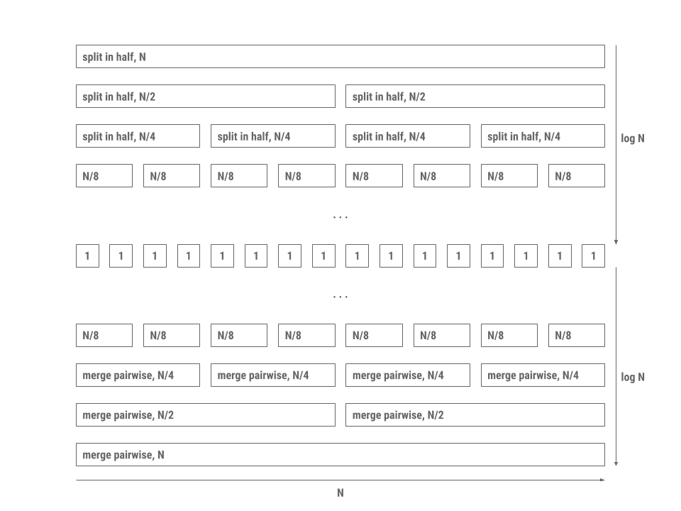
Note that this is a good visualization of all the work that is being done but does not visually represent the order of the recursive calls being done. Merge sort will recursively call merge on the first partition until it reaches the base case of a single element, and then will begin the merge step (which will build the problem back up).

Runtime and Stability

To evaluate the runtime, we will be using the merge sort image above.

We begin with the entire collection, which is of size \(N\). Splitting this collection in half will require \(N\) time, resulting in two \(\frac{N}{2}\) sized collections. We will then call merge sort on both of these \(\frac{N}{2}\) sized collections, which will result in two \(\frac{N}{2}\) time operations to split their respective collections. This totals in \(N\) time, meaning that there is \(N\) work done at that level. This pattern will repeat for each level that does this split operation, so there will be a total of \(N\) work for each of the \(\log N\) levels of splitting.

Once we reach the base case of empty or one-element collections, we can then start merging our list back together. Every single recursive call will merge the two sorted half-collections of size \(\frac{k}{2}\) in \(k\) time (iterate through each half-collection and combine the half-collections into a whole collection). Thus, the same idea will occur as it did for splitting: each level will take \(N\) work, and there will be a total of \(\log N\) levels of merging.

In total, we will have \(2 \log N\) levels with each level doing work proportional to \(N\). The total runtime of merge sort will be \(\Theta(N \log N)\).

Merge sort is stable as long as we make sure when merging two halves together that we favor equal elements in the left half before those in the right half.

Worksheet 1.1(d): Merge sort

Complete this problem on the worksheet. Write out what the array looks like after each pass of merge sort (you can assume that we have recursed down to the single item partitions and are in the process of merging the partitions back together pairwise. You should draw merge sort level by level). Make sure to double check with your TA if you have any questions!

Quicksort

Our next example of dividing and conquering is the quicksort algorithm, which proceeds as follows:

1. Split the collection to be sorted into three collections by partitioning around a pivot element. One collection consists of elements smaller than the pivot, the second collection consists of elements equal to the pivot, and the third consists of elements greater than the pivot.
2. Recursively call quicksort on the each collection.
3. Merge the sorted collections by concatenation.

Specifically, this version of quicksort is called “three-way partitioning quicksort” due to the three partitions that the algorithm makes on every call.

Note: this sort is very similar to merge sort in its general structure, but the small differences in the algorithm will result in some interesting analyses later!

Here’s an example of how this might work, sorting an array containing 3, 1, 4, 5, 9, 2, 8, 6. The blue boxed numbers indicate the pivot selection for each partition.

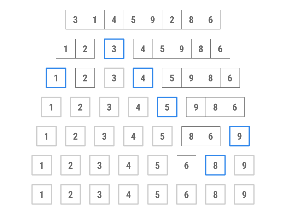
1. Choose 3 as the pivot. (We’ll explore how to choose the pivot shortly.)
2. Put 4, 5, 9, 8, and 6 into the “large” collection and 1 and 2 into the “small” collection. No elements go in the “equal” collection.
3. Sort the large collection into 4, 5, 6, 8, 9; sort the small collection into 1, 2; combine the two collections with the pivot to get 1, 2, 3, 4, 5, 6, 8, 9.

Note that while this is a good visualization of how this sort will work, this image does not display the order of the recursive calls that are made. On the third line, it looks like the smaller (1, 2) and larger (4, 5, 9, 8, 6) partitions are being dealt with simultaneously, though in the actual run of the algorithm, one partition’s call to quicksort would have to complete before the other partitions can begin their calls to quicksort.

Quicksort using three-way partitioning is stable since we create auxiliary arrays to hold each partition. We add elements in the order we come across them as we are partitioning, so relative ordering of equal elements will not change.

Worksheet 1.2: Quicksort

Complete this problem on the worksheet. Write out what the array looks like after each pass of quicksort (see the image above for an example of what you should be writing down). Make sure to double check with your TA if you have any questions!

Note: We haven’t discussed pivot selection yet, so just pick the first element as your pivot!

Runtime

First, let’s consider the best-case scenario where each partition divides a range optimally in half. In total, we would have a total of \(\log N\) levels. Every level will consist of partitioning all the elements, recursively calling quicksort, and merging the partitions back together, which would result in work proportional to \(N\). Thus, the total time is proportional to \(N \log N\).

However, quicksort is faster in practice and tends to have better constant factors (which are usually simplified away in most runtime analyses). To see this, let’s examine exactly how quicksort works.

We know concatenation in a linked list can be done in constant time or linear time if it’s an array. Partitioning can be done in time proportional to the number of elements \(N\). If the partitioning is optimal and splits each range more or less in half, we have a similar logarithmic division of levels downward like in merge sort. On each division, we still do the same linear amount of work as we need to decide whether each element is greater or less than the pivot.

However, once we’ve reached the base case, we don’t need as many steps to reassemble the sorted collection. Remember that with merge sort, while each list of one element is sorted with respect to itself, the entire set of one-element lists is not necessarily in order which is why there are \(\log N\) steps to merge upwards in merge sort. This isn’t the case with quicksort as each element is in order. Thus, merging in quicksort is simply one level of linear-time concatenation.

Unlike merge sort, quicksort has a worst-case runtime different from its best-case runtime. Suppose we always choose the 0th element of a partition as the pivot. If our array was already sorted or reverse-sorted, this would create one partition with 0 elements and another partition with the rest of the elements. When we recursively quicksort the partition with elements, we would again create one partition with 0 elements and another partition with the rest of the elements. Does this special case of quicksort remind you of any other sorting algorithm we’ve discussed in this lab? That’s right, it’s selection sort!

We know that selection sort’s runtime if \(\Theta(N^2)\), so we know that quicksort’s worst case runtime is also \(\Theta(N^2)\). Quicksort’s worst case runtime is worse than merge sort’s worst case!

Average Case

The average case runtime of quicksort depends on the pivot chosen.

In the best case, the pivot chosen would create two equal-sized partitions (the pivot is the median value), each with 50% of the elements. (It is non-trivial find the median element of an array, so guaranteeing this case is hard.)

In the worst case, the pivot chosen would be the smallest or largest element of that partition, creating two partitions, one with 0% of the elements and another with near 100% of the elements.

But what happens in the “average” case?

Assuming the choice of pivot is uniformly random, the split obtained is uniform random between 50/50 and 0/100. That means in the average case, we expect a split of 25/75. This gives a recursion tree of height \(\log_\frac{4}{3}(N)\) where each level does \(N\) work. Then quicksort still takes \(\Theta(N \log N)\) time in the average case.

How often does the bad-pivot case come up if we pick pivots uniformly at random? If we consider half of the array as bad pivots, as the array gets longer, the probability of picking a bad pivot for every recursive call to quicksort exponentially decreases.

For an array of length 30, the probability of picking all bad pivots is \(\frac{1}{2}^{30} = 9.3 \cdot 10^{-10}\), which is approximately the same as winning the Powerball: \(3.3 \cdot 10^{-9}\).

For an array of length 100, the probability of picking all bad pivots, \(7.8 \cdot 10^{-31}\), is so low that if we ran quicksort every second for 100 billion years, we’d still have a significantly better chance trying to win the lottery in one ticket.

Of course, there’s the chance you pick something in between, and the analysis can get far more complicated, especially with variants of quicksort. For practical purposes, we can treat quicksort like it’s in \(\Theta(N \log N)\).

Quicksort in Practice

Finding the exact median of our elements may take so much time that it may not help the overall runtime of quicksort at all. It may be worth it to choose an approximate median, if we can do so really quickly. Options include picking a random element, or picking the median of the first, middle, and last elements. These will at least avoid the worst case we discussed above.

In practice, quicksort turns out to be the fastest of the general-purpose sorting algorithms we have covered so far. For example, it tends to have better constant factors than that of merge sort. For this reason, Java uses this algorithm for sorting arrays of primitive types, such as ints or floats. With some tuning, the most likely worst-case scenarios are avoided, and the average case performance is excellent.

Here are some improvements to the quicksort algorithm as implemented in the Java standard library:

• When there are only a few items in a sub-collection (near the base case of the recursion), insertion sort is used instead.
• For larger arrays, more effort is expended on finding a good pivot.
• Various machine-dependent methods are used to optimize the partitioning algorithm and the swap operation.
• Dual pivots

For object types, however, Java uses a hybrid of merge sort and insertion sort called “Timsort” instead of quicksort. Can you come up with an explanation as to why? Hint: Think about stability!

Exercise: Sorts.java

Now, let’s implement a few sorts! We won’t implement all of them; only insertion sort, merge sort, and quicksort.

After each sort, be sure to take a look at SortsTest.java, which contains a suite of randomized tests similar to the ones used in the autograder. Remember you are free to change any parts of the test, especially if you want to change the NUM_ITEMS_TO_SORT to sort smaller examples that might be easier to debug.

insertionSort

We have provided code for insertion sort on an array. Now, let’s try writing insertion sort for linked lists!

First, implement insertionSort in Sorts.java. This method should be destructive and iterative.

Run the test in SortsTest.java and make sure you pass the test before moving on!

mergeSort

Next, fill out the mergeSort method in Sorts.java. This method should be destructive and recursive.

Run the test in SortsTest.java and make sure you pass the test before moving on!

quickSort

Some of the code is missing from the quickSort method in Sorts.java. Fill in the function to complete the quicksort implementation. This method should be destructive and recursive.

Use the generator object to help you randomly choose a pivot element to use.

Run the test in SortsTest.java and make sure you pass the test before moving on!

Worksheet 1.3: Runtime and Stability Table

Complete this table with the runtimes and stability of each of the sorts we learned. Make sure you know why the runtimes and stability are the way they are and know what assumptions are being made about each sort (such as a sort’s implementation when it comes to determining stability).

If you have any questions, be sure to check with your TA!

Conclusion

Summary

In this lab, we learned about different comparison-based algorithms for sorting collections. Within comparison-based algorithms, we examined two different paradigms for sorting:

1. Sorts like insertion sort, selection sort, and heapsort which demonstrated algorithms that maintained a sorted section and moved unsorted elements into this sorted section one-by-one. With optimization like heap sort or the right conditions (relatively sorted list in the case of insertion sort), these simple sorts can be fast!
2. Divide and conquer sorts like merge sort and quicksort. These algorithms take a different approach to sorting: we instead take advantage of the fact that collections of one element are sorted with respect to themselves. Using recursive procedures, we can break larger sorting problems into smaller subsequences that can be sorted individually and quickly recombined to produce a sorting of the original collection.

Here are several online resources for visualizing sorting algorithms. If you’re having trouble understanding these sorts, use these resources as tools to help build intuition about how each sort works.

• VisuAlgo
• Sorting.at
• Sorting Algorithms Animations
• USF Comparison of Sorting Algorithms
• AlgoRhythmics: sorting demos through folk dance including insertion sort, selection sort, merge sort, and quicksort

Deliverables

To get credit for this lab:

• Turn in the worksheet to your TA by the end of lab.
• Complete the following methods in Sorts.java:
  • insertionSort
  • mergeSort
  • quickSort