Introduction

As usual, pull the files from the skeleton and make a new IntelliJ project.

In the last lab, we learned about comparison-based sorts, all with varying runtimes. It’s not always clear which sort we should use, since each sort has it’s own strengths and weaknesses. However, notice that none of the sorts had a worst case runtime that was better than \(\Theta(N \log N)\). Is it possible to do better than this in the worst case for these comparison-based sorts?

A Sorting Lower Bound

Suppose we have a scrambled array of \(N\) numbers, with each number from \(1\) to \(N\) occurring once. How many possible orders can the numbers be in?

The answer is \(N!\), where \(N! = 1 * 2 * 3 * \dots * (N - 2) * (N - 1) * N\). Here’s why: the first number in the array can be anything from \(1\) to \(N\), yielding \(N\) possibilities. Once the first number is chosen, the second number can be any of the remaining \(N - 1\) numbers, so there are \(N(N - 1)\) possible choices of the first two numbers. The third number can be any of the remaining \(N - 2\) numbers, yielding \(N * (N - 1) * (N - 2)\) possibilities for the first three numbers. We can continue this reasoning to get a total of \(N!\) arrangements of the numbers \(1\) to \(N\).

Each different order is called a permutation of the numbers, and there are \(N!\) possible permutations.

Observe that if \(N\) > 0,

\[N! = 1 * 2 * \dots * (N - 1) * N \leq N * N * N * \dots * N * N * N = N^N\]

and (supposing \(N\) is even)

\[N! = 1 * 2 * \dots * (N - 1) * N \geq \frac{N}{2} * (\frac{N}{2} + 1) * \dots * (N - 1) * N \geq \frac{N}{2}^{\frac{N}{2}}\]

so

\[\frac{N}{2}^{\frac{N}{2}} \leq N! \leq N^N\]

Now let’s look at the logarithms of both these values:

\[\log(\frac{N}{2}^{\frac{N}{2}}) = \frac{N}{2} \log (\frac{N}{2})\] \[\log (N^N) = N \log N\]

Both of these values are in \(\Theta(N \log N)\). Hence, \(\log(N!)\) is also in \(\Theta(N \log N)\).

A comparison-based sort is one in which all decisions are based on comparing keys (generally done by “if” statements). All actions taken by the sorting algorithm are based on the results of a sequence of true/false questions. All of the sorting algorithms we have studied so far are comparison-based.

Suppose that two computers run the same sorting algorithm at the same time on two different inputs. Suppose that every time one computer executes an “if” statement and finds it true, the other computer executes the same “if” statement and also finds it true; likewise, when one computer executes an “if” and finds it false, so does the other. Then both computers perform exactly the same data movements (e.g. swapping the numbers at indices i and j) in exactly the same order, so they both permute their inputs in exactly the same way.

A correct sorting algorithm must generate a different sequence of true/false answers for each different permutation of \(1\) to \(N\), because it takes a different sequence of data movements to sort each permutation. There are \(N!\) different permutations, thus \(N!\) different sequences of true/false answers.

If a sorting algorithm asks \(d\) true/false questions, it generates less than or equal to \(2^d\) different sequences of true/false answers. If it correctly sorts every permutation of \(1\) to \(N\), then \(N! \leq 2^d\), so \(\log_2 (N!) \leq d\). We know that \(\log_2(N!)\) is in \(\Theta(N \log N)\), so \(\Theta(N \log N) \leq d\). This means that \(d\) is in \(\Omega(N \log N)\), which implies that the algorithm spends \(\Omega(d)\) time (in other words, \(\Omega(N \log N)\) time) asking these \(d\) questions. Hence,

EVERY comparison-based sorting algorithm takes \(\Omega(N \log N)\) time in the worst-case.

This is an amazing claim, because it doesn’t just analyze one algorithm. It says that of the thousands of comparison-based sorting algorithms that haven’t even been invented yet, not one of them has any hope of beating \(O(N \log N)\) time for all inputs of length \(N\).

In the worst case, a comparison-based sort (with 2-way decisions) must take at least \(\Theta(N \log N)\) time. But what if instead of making a 2-way true/false decision, we make a k-way decision?

A Linear Time Sort

Suppose we have an array of a million Strings, but we happen to know that there are only three different varieties of Strings in it: “cat”, “dog”, and “person”. We want to sort this array to put all the cats first, then all the dogs, then the people. How would we do it? We could use merge sort or quicksort and get a runtime proportional to \(N \log N\), where \(N\) is roughly one million, but can we do better?

We can propose an algorithm called counting sort. For the above example, it works like this:

1. First, let’s create an integer array of size three called the counts array. This array will count the total number of each String, where “cat” will correspond to counts[0], “dog” will correspond to counts[1], and “person” will correspond to counts[2].

2. Then, let’s iterate through the input array and update the counts array. Every time you find “cat”, “dog”, or “person”, increment counts[0], counts[1], and counts[2] by 1 respectively. As an example, the result could be this: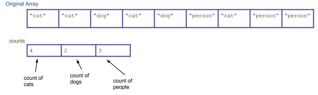

3. Next, let’s create a new String array called sorted that will eventually be your sorted array.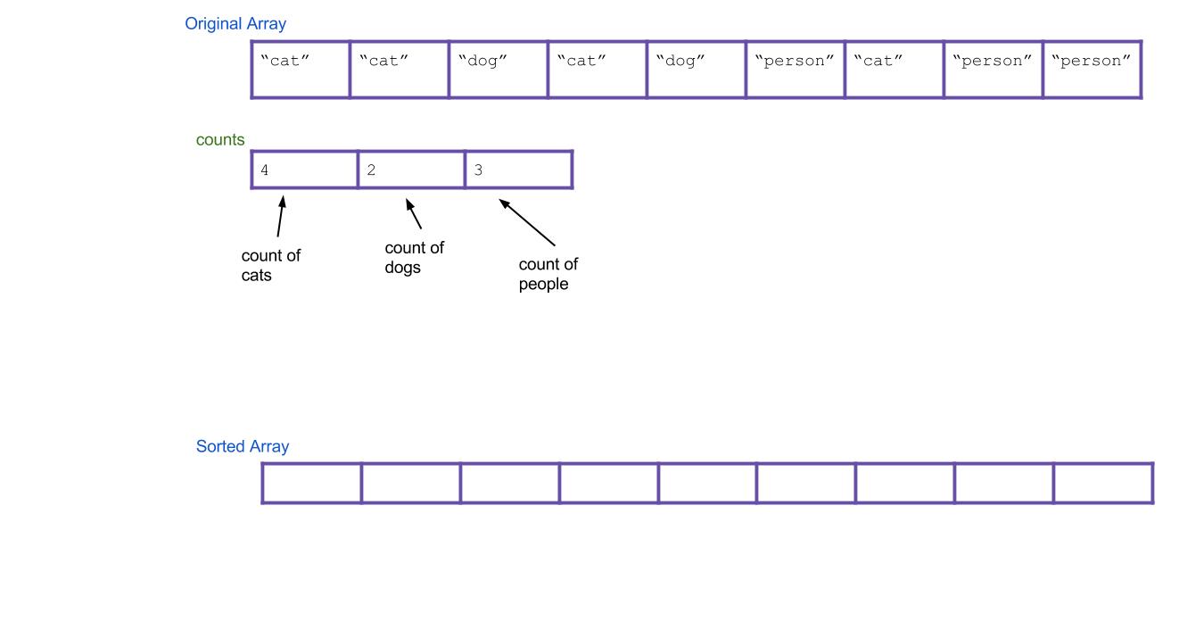

4. Now, based on our counts array, can we tell where the first “dog” would go in the new array? How about the first “person”? To do this, we should create a new array called starts that holds this information. We can get this by scanning through the counts array and finding the total number of items to the left of index i. For our example, the result is: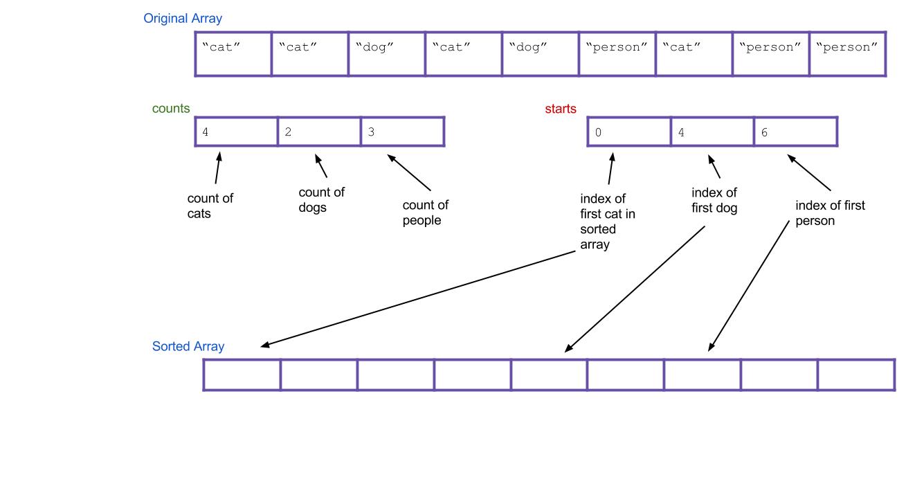

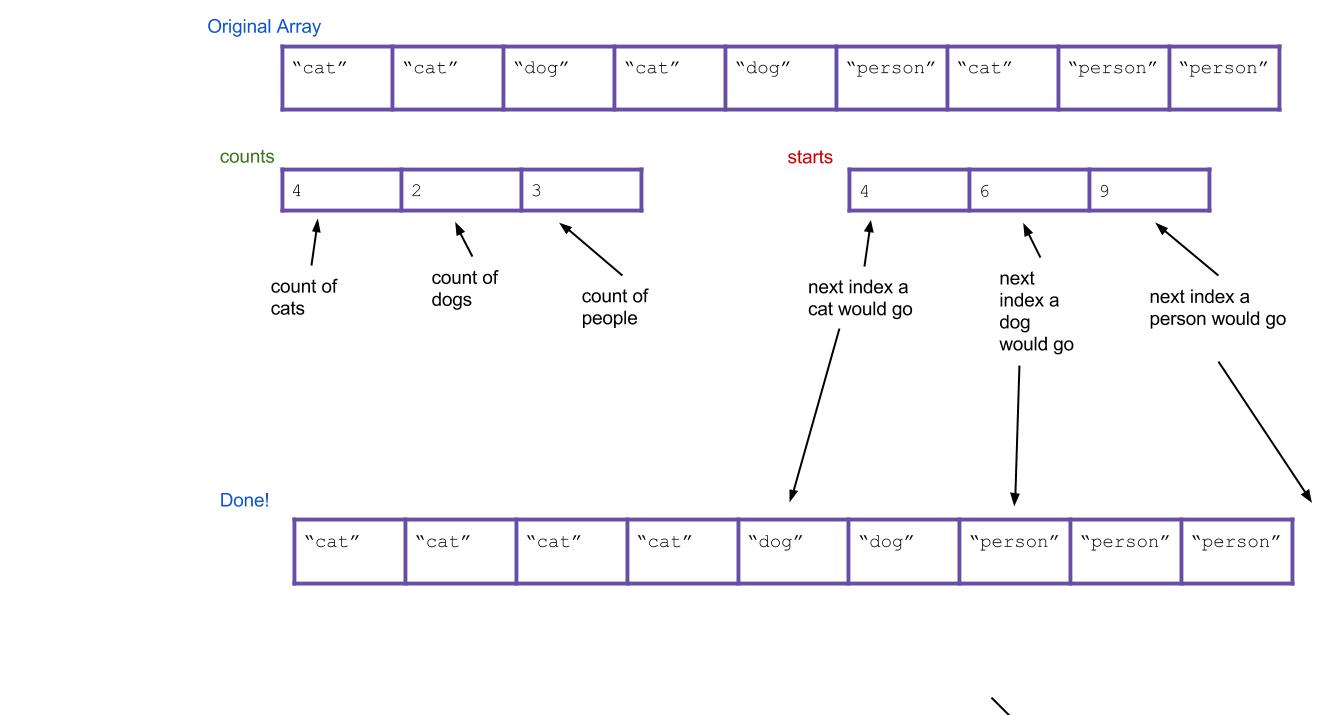
5. Now iterate through all of our Strings, and put them into the right spot. When we find the first “cat”, it goes in sorted[starts[0]]. When we find the first “dog”, it goes in sorted[starts[1]]. What about when we find the second “dog”? It should go in sorted[starts[1]+1]! Or, an alternative: we can just increment starts[1] every time we put a “dog”. Then, the next “dog” will always go in sorted[starts[1]].

Here’s what everything would look like after completing the algorithm. Notice that the values of starts have been incremented along the way.

This written explanation of counting sort may seem complicated, so take a look at this counting sort visualization that might make this algorithm more intuitive. Note that this visualization combines the counts and starts arrays into one, which is why there is only two additional arrays rather than 3 that we have in our example.

Worksheet 1.1: Counting Sort

Let’s try this on paper! Complete this exercise on your worksheet.

Make sure you write down what all the arrays look like after the run of counting sort is over (including any changes we make to starts that occurs in Step 5)!

Runtime

Now that we’re more comfortable with counting sorts, let’s analyze the runtime.

Let’s assume that \(N\) is the number of items in the array, and \(R\) is the variety of possible items. In the example above with “cat”, “dog”, and “person”, \(R\) was 3. In the example from the worksheet, \(R\) was 10 (these were the digits 0, 1, 2, 3, 4, 5, 6, 7, 8, and 9).

To do counting sort, we will make one pass over the array (\(N\) work) to populate our counts array. Then, we will make one pass over our counts array (\(R\) work) to populate the starts array. Then, we will make one more pass over our array (\(N\) work) to populate the output array. In total, we will do \(N + R + N\) work, which simplifies to \(\Theta(N + R)\).

Wow, look at that runtime! Does this mean counting sort is a strict improvement from quicksort? Not quite; counting sort has two major weaknesses:

• It can only be used to sort discrete values.
• It will be very slow (and possibly even fail) if \(R\) is too large, because creating the intermediate counts array of size \(R\) will be too slow or infeasible.

The latter point turns out to be a fatal weakness for counting sort. The range of all possible integers in Java is just too large for counting sort to be practical in general circumstances.

Suddenly, counting sort seems completely useless. However, with some modifications that we’ll see in a little bit, we can come up with a pretty good sorting algorithm!

Radix Sort

Aside from counting sort, all the sorting methods we’ve seen so far are comparison-based. This means they use comparisons to determine whether two elements are out of order. We also saw the proof that any comparison-based sort needs at least \(\Theta(N \log N)\) comparisons to sort \(N\) elements in the worst case. However, there are sorting methods that don’t depend on comparisons that allow sorting of \(N\) elements in time proportional to \(N\). Counting sort was one, but turned out to be impractical.

However, we now have all the ingredients necessary to describe radix sort, another linear-time non-comparison sort that can be practical.

Let’s first define the word, radix. The radix of a number system is the number of values a single digit can take on (also called the base of a number). Binary numbers form a radix-2 system; decimal notation is radix-10; the English alphabet has 26 letters and is radix-26. Radix sorts will examine elements in passes, and a radix sort might have one pass for the rightmost digit, one for the next-to-rightmost digit, and so on.

We’ll now describe radix sort in detail. We actually already described a procedure similar to radix sort when talking about sorting animals in the last lab. In radix sort, we will pretend each digit is a separate key, and then we sort on all the keys at once, with the higher digits taking precedence over the lower ones.

Here are two good strategies to approach sorting on multiple keys:

• First sort everything on the least important key. Then sort everything on the next key. Continue, until you reach the highest key. Note: This strategy requires the sorts to be stable.
• First sort everything on the high key. Group all the items with the same high key into buckets. Recursively radix sort each bucket on the next highest key. Concatenate your buckets back together.

Here’s an example of using the first strategy. Imagine we have the following numbers we wish to sort:

356, 112, 904, 294, 209, 820, 394, 810

First we sort them by the first digit:

820, 810, 112, 904, 294, 394, 356, 209

Then we sort them by the second digit, keeping numbers with the same second digit in their order from the previous step:

904, 209, 810, 112, 820, 356, 294, 394

Finally, we sort by the third digit, keeping numbers with the same third digit in their order from the previous step:

112, 209, 294, 356, 394, 810, 820, 904

All done!

Hopefully it’s not hard to see how these can be extended to more than three digits. This strategy is known as LSD radix sort. The second strategy is called MSD radix sort. LSD and MSD stand for least significant digit and most significant digit respectively, reflecting the order in which the digits are considered.

Here’s some pseudocode for the first strategy:

public static void lsdRadixSort(int[] arr) {
    for (int d = 0; d < numDigitsInAnInteger; d++) {
        stableSortOnDigit(arr, d);
    }
}

(the 0th digit is the smallest digit, or the one furthest to the right in the number)

Radix Sort’s Helper Method

Notice that both LSD and MSD radix sort call another sort as a helper method (in LSD’s case, it must be a stable sort). Which sort should we use for this helper method? Insertion sort? Merge sort? Those would work. However, notice one key property of this helper sort: It only sorts based on a single digit. And a single digit can only take 10 possible values (for radix-10 systems). This means we’re doing a sort where the variety of things to sort is small. Do we know a sort that’s good for this? It’s counting sort! Counting sort turns out to be useful as a helper method to radix sort when it comes to sorting the elements by a particular digit.

Worksheet 1.2: LSD Radix Sort

Complete this exercise on the worksheet, which runs LSD radix sort on a given array (where LSD stands for least significant digit). Remember that the least significant digit is the rightmost digit.

Worksheet 1.3: MSD Radix Sort

Now that we’ve gotten practice with LSD radix sort, let’s move onto the next problem. Complete this exercise on the worksheet, which runs MSD radix sort on a given array (where MSD stands for most significant digit). Remember that the most significant digit is the leftmost digit.

Note: Remember that MSD radix sort is implemented recursively, where we will recursively sort each of the “buckets”. The worksheet’s levels don’t represent this recursive property very well, but know that MSD radix sort uses recursion to sort each bucket and then concatenates them in the end!

Worksheet 1.4: Runtimes

Before we try this exercise on the worksheet, let’s analyze the runtimes together.

LSD Radix Sort

Let’s examine the pseudocode given for LSD radix sort. From this, we can tell that its runtime is proportional to numDigitsInAnInteger * (the runtime of stableSortOnDigit).

Let’s call numDigitsInAnInteger the variable \(W\), which is the max number of digits that an integer in our input array has. Next, remember that we decided stableSortOnDigit is really counting sort, which has runtime proportional to \(N + R\), where \(R\) is the number of possible digits (radix), in this case

1. This means the total runtime of LSD radix sort is \(\Theta(W(N + R))\)!

MSD Radix Sort

Now, what is the runtime for MSD radix sort? How does it differ from LSD radix sort’s runtime?

Hint: Unlike LSD radix sort, it will be important to distinguish best-case and worst-case runtimes for MSD.

Complete this exercise by filling out the table on the worksheet! Be sure to ask your TA any questions that you have about this part before moving on.

Exercise: Distribution Sorts

We will now be implementing counting sort and LSD radix sort in DistributionSorts. We have also included DistributionSortsTest, which contains some tests that are similar to the autograder tests. Make sure to use these local tests if you need to debug, rather than submitting to the autograder!

Exercise 1: countingSort

Implement the countingSort method, which should perform counting sort on the input array. countingSort should modify the original array passed in, and therefore is destructive. Assume the only integers the input array will contain are 0, 1, 2, 3, 4, 5, 6, 7, 8, and 9.

Refer to the steps above about counting sort if you’re having trouble with this method!

After you’re done implementing this method, make sure to run the tests in DistributionSortsTest to double check your work!

Exercise 2: lsdRadixSort

Complete the lsdRadixSort method in by implementing the countingSortOnDigit method. You won’t be able to reuse your countingSort from before verbatim because you need a method to do counting sort only considering one digit, but you will be able to use something very similar.

Disclaimer: Radix sort is commonly implemented at a lower level than base-10, such as with bits (base-2) or bytes (base-16). This is because everything on your computer is represented with bits. Through bit operations, it is quicker to isolate a single bit or byte than to get a base-10 digit. However, because we don’t teach you about bits in this course, you should do your LSD radix sort in base-10 because these types of numbers should be more familiar to you.

If you are up for a challenge, feel free to figure out how to implement radix sort using bytes and bit-operations (you will want to look up bit masks and bit shifts).

Advanced Runtime and Radix Selection

Let’s go back and analyze the LSD radix sort runtime (despite the best-case runtime of MSD radix sort, LSD radix sort is typically better in practice). You may have noticed that there’s a balance between \(R\), the number of digits (also known as the radix), and \(W\), the number of passes needed. In fact, they’re related in this way: let us call \(L\) the length of the longest number in digits. Then \(R \cdot W\) is proportional to \(L\).

For example, let’s say that we have the radix-10 numbers 100, 999, 200, 320. In radix-10, they are all of length 3, and we would require 3 passes of counting sort. However, if we took those same numbers and now use radix-1000, then we examine more of the numbers, all 3 of the base-10 digits, and we only require one pass of counting sort. In fact, in radix-1000, the numbers we used are only of length 1.

In fact, in practice we shouldn’t be using decimal digits at all - radixes are typically a power of two. This is because everything is represented as bits, and as mentioned previously, bit operators are significantly faster than modulo operators, and we can pull out the bits we need if our radix is a power of two.

Without further knowledge of bits, it’s difficult to analyze the runtime further, but we’ll proceed anyways - you can read up on bits on your own time. Suppose our radix is \(R\). Then each pass of counting sort inspects \(\lg R\) bits; if the longest number has b bits, then the number of passes \(D = \frac{b}{\lg R}\). This doesn’t change our runtime of LSD radix sort from \(\Theta(W \cdot (N + R))\).

Here’s the trick: we can choose \(R\) to be larger than in our exercises (10). In fact, let’s choose \(R\) to be in \(O(N)\) (that way each pass counting sort will run in \(O(N)\)). We want \(R\) to be large enough to keep the number of passes small. Thus the number of passes needed becomes \(W \in O(\frac{b}{\lg (N)})\).

This means our true runtime must be \(O(N)\) if \(b\) is less than \(\lg N\) or otherwise \(O(N \cdot \frac{b}{\lg N})\), (plug our choices for \(W\) and \(R\) into the runtime for LSD radix sort above to see why that’s the case). For very typical things we might sort, like ints, or longs, \(b\) is a constant, and thus radix sort is guaranteed linear time. For other types, as long as \(b\) is in \(O(\lg N)\), this remains in guaranteed linear time. It’s worth noting that because it takes \(\lg N\) bits to represent N items, this is a very reasonable model of growth for typical things that might be sorted - as long as your input is not distributed scarcely.

Conclusion

Linear-time sorts have their advantages and disadvantages. While they have fantastic speed guarantees theoretically, the overhead associated with a linear time sort means that for input lists of shorter length, low overhead comparison based sorts like quicksort can perform better in practice. For more specialized mathematical computations, like in geometry, machine learning, and graphics, for example, radix sort finds use.

In modern libraries like Java and Python’s standard library, a new type of sort, TimSort, is used. It’s a hybrid sort between merge sort and insertion sort that also has a linear-time guarantee - if the input data is sorted, or almost sorted, it performs in linear time. In practice, on real-world inputs, it’s shown to be very powerful and has been a staple in standard library comparison sorts.

Deliverables

To receive credit for this lab, complete the following methods in DistributionSorts:

• countingSort
• countingSortOnDigit

Credit

Credit to Jonathan Shewchuk for his notes on the lower bound of comparison-based sorting algorithms.