Introduction

As we discussed in previous labs, there are a few ADT’s that are critical building blocks to more complex structures. Today, we will explore an implementation of the Set ADT called disjoint sets. Then, we will change subjects to expand upon our knowledge of graphs with minimum spanning trees and how to find them.

As usual, pull the files from the skeleton and make a new IntelliJ project.

Disjoint Sets

Suppose we have a collection of companies that have gone under mergers or acquisitions. We want to develop a data structure that allows us to determine if any two companies are in the same conglomerate. For example, if company X and company Y were originally independent but Y acquired X, we want to be able to represent this new connection in our data structure. How would we do this? One way we can do this is by using the disjoint sets data structure.

The disjoint sets data structure represents a collection of sets that are disjoint, meaning that any item in this data structure is found in no more than one set. When discussing this data structure, we often limit ourselves to two operations, union and find, which is also why this data structure is sometimes called the union-find data structure. We will be using these two names interchangeably for the remainder of this lab.

The union operation will combine two sets into one set. The find operation will take in an item, and tell us which set that item belongs to. With this data structure, we will be able to keep track of the acquisitions and mergers that occur!

Let’s run through an example of how we can represent our problem using disjoint sets with the following companies:

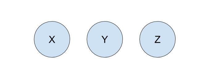
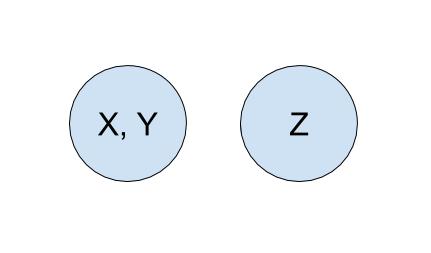
To start off, each company is in its own set with only itself and a call to find(X) will return \(X\) (and similarly for all the other companies). If \(Y\) acquired \(X\), we will make a call to union(X, Y) to represent that the two companies should now be linked. As a result, a call to find(X) will now return \(Y\), showing that \(X\) is now a part of \(Y\). The unioned result is shown below.

Quick Find

For the rest of the lab, we will work with non-negative integers as the items in our disjoint sets.

In order to implement disjoint sets, we need to know the following:

• What items are in each set
• Which set each item belongs to

One implementation we can do involves keeping an array that details just that. In our array, the index will represent the item (hence non-negative integers) and the value at that index will represent which set that item belongs to. For example, if our set looked like this,

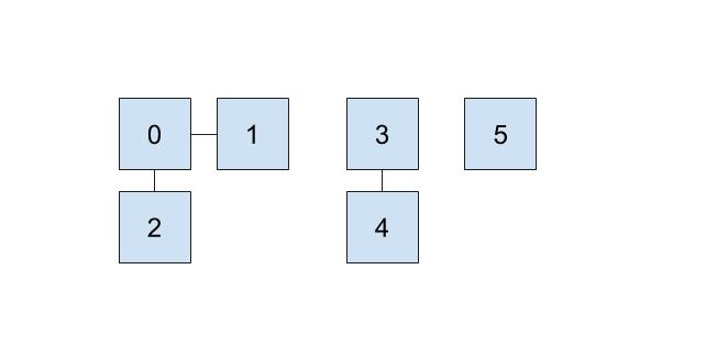
then we could represent the connections like this:

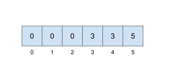
Here, we will be choosing the smallest number of the set to represent the face of the set, which is why the set numbers are 0, 3, and 5.

This approach uses the quick-find algorithm, prioritizing the runtime of the find operation but making the union operations slow. To implement the find operation, you will just need to access the item at the correct index which can be done in \(\Theta(1)\) time! However, in order to correctly perform a union operation, we will need to iterate through the entire array, resulting in a \(\Theta(N)\) operation.

Quick Union

Suppose we prioritize making the union operation fast instead. One way we can do that is that instead of representing each set as we did above, we will think about each set as a tree.

This tree will have the following qualities:

• the nodes will be the items in our set,
• each node only needs a reference to its parent rather than a direct reference to the face of the set, and
• the top of each tree (we refer to this top as the “root” of the tree) will be the face of the set it represents.

In the example from the beginning of lab, \(Y\) would be the face of the set represented by \(X\) and \(Y\), so \(Y\) would be the root of the tree containing \(X\) and \(Y\).

How do we modify our data structure from above to make this quick union? We will just need to replace the set references with parent references! The indices of the array will still correspond to the item itself, but we will put the parent references inside the array instead of direct set references. If an item does not have a parent, that means this item is the face of the set and we will instead record the size of the set. In order to distinguish the size from parent references, we will record the size, \(s\), of the set as \(-s\) inside of our array.

When we union(u, v), we will find the set that each of the values belong to (the roots of their respective trees), and make one the child of the other. If u and v are both the face of their respective sets and in turn the roots of their own tree, union(u, v) is a fast \(\Theta(1)\) operation because we just need to make the root of one set connect to the root of the other set!

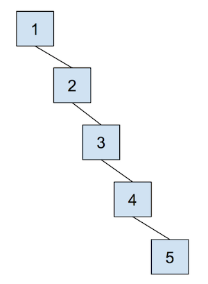
The cost of a quick union, however, is that find can now be slow. In order to find which set an item is in, we must jump through all the parent references and travel to the root of the tree, which is \(\Theta(N)\) in the worst case. Here’s an example of a tree that would lead to the worst case runtime, which we often refer to as “spindly”:

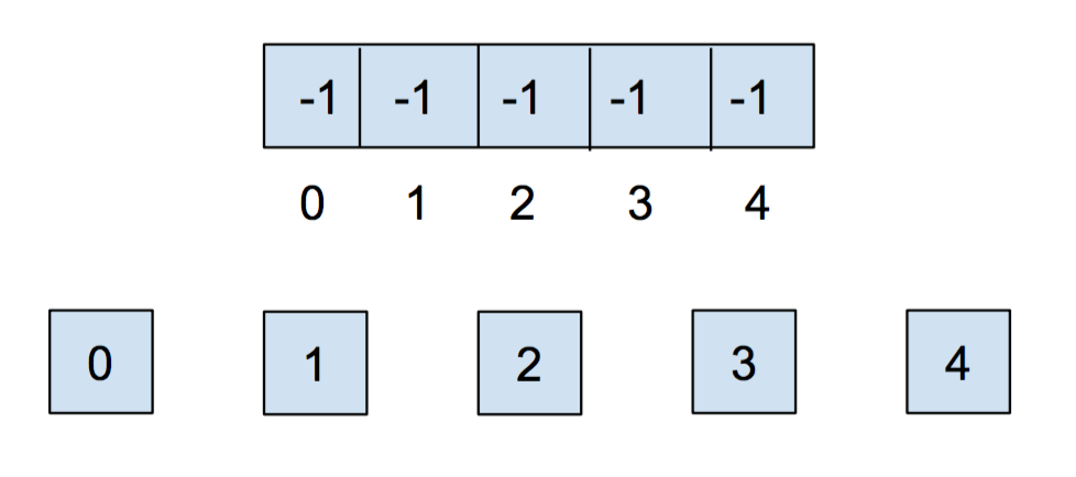
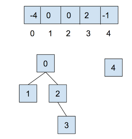
In addition, union-ing two leaves could lead to the same worst case runtime as find because we would have to first find the sets that each of the leaves belong to before completing union operation. We will soon see some optimizations that we can do in order to make this runtime faster, but let’s go through an example of this quick union data structure first. The array representation of the data structure is shown first, followed by the abstract tree representation of the data structure.

Initially, each item is in its own set, so we will initialize all of the elements in the array to -1.

After we call union(0,1) and union(2,3), our array and our abstract representation look as below:

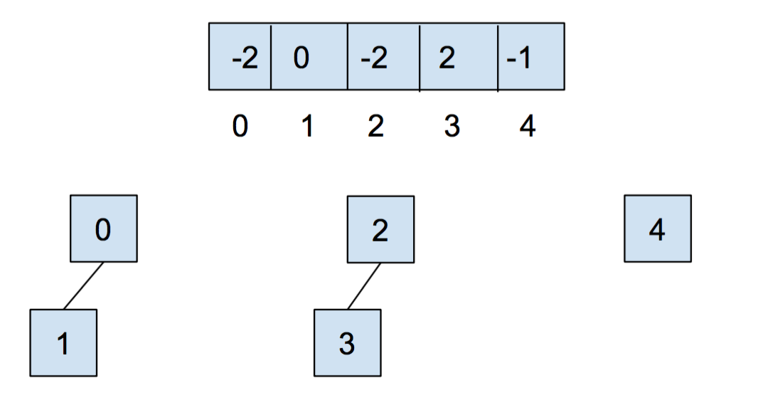
After calling union(0,2), they look like:

Now, let’s combat the shortcomings of this data structure with the following optimizations.

Weighted Quick Union

The first optimization that we will do for our quick union data structure is called “union by size”. This will be done in order to keep the trees as shallow as possible and avoid the spindly trees that result in the worst-case runtimes. When we union two trees, we will make the smaller tree (the tree with less nodes) a subtree of the larger one, breaking ties arbitrarily. We call this weighted quick union.

Because we are now using “union by size”, the maximum depth of any item will be in \(\Theta(\log N)\), where \(N\) is the number of items stored in the data structure. This is a great improvement over the linear time runtime of the unoptimized quick union. Some brief intuition for this depth is because the depth of any element \(x\) only increases when the tree \(T_1\) that contains \(x\) is placed below another tree \(T_2\). When that happens, the size of the resulting tree will be at least double the size of \(T_1\) because \(size(T_2) \ge size(T_1)\). The tree that contains only \(x\) can double its size at most \(\log N\) times until we have reached a total of \(N\) items.

Path Compression

Even though we have made a speedup by using a weighted quick union data structure, there is still yet another optimization that we can do. What would happen if we had a tall tree and called find repeatedly on the deepest leaf? Each time, we would have to traverse the tree from the leaf to the root.

A clever optimization is to move the leaf up the tree so it becomes a direct child of the root. That way, the next time you call find on that leaf, it will run much more quickly. Remember that we do not care if a node has a certain parent; we care more about general connectivity (and therefore only what the root is), which is why we can move the leaf up to be a child of the root without losing important information about our disjoint sets structure.

An even more clever idea is that we could do the same thing to every node that is on the path from the leaf to the root, connecting each node to the root as we traverse up the tree. This optimization is called path compression. Once you find an item, path compression will make finding it (and all the nodes on the path to the root) in the future faster.

The runtime for any combination of \(f\) find and \(u\) union operations takes \(\Theta(u + f \alpha(f+u,u))\) time, where \(\alpha\) is an extremely slowly-growing function called the inverse Ackermann function. And by “extremely slowly-growing”, we mean it grows so slowly that for any practical input that you will ever use, the inverse Ackermann function will never be larger than 4. That means for any practical purpose, a weighted quick union data structure with path compression has find operations that take constant time on average!

You can visit this link here to play around with disjoint sets.

Worksheet 1.1: WQUPC

Complete this exercise on the worksheet that gives practice with the weighted quick union with path compression data structure!

Worksheet 1.2: Runtimes

Complete this exercise on the worksheet that summarizes all the runtimes that we have learned so far.

Remember that union will often call find, so make sure to take that into account in your runtimes!

Exercise: UnionFind

We will now implement our own disjoint sets data structure. When you open up UnionFind.java, you will see that it has a number of method headers with empty implementations.

Read the documentation to get an understanding of what methods need to be filled out. Remember to implement both optimizations discussed above, and take note of the tie-breaking scheme that is described in union method’s comments. You will also want to ensure that the inputs to your functions are within bounds; otherwise you should throw an IllegalArgumentException.

Note: Many other tie-breaking schemes could be used, but we will choose this one for autograding purposes.

Discussion: UnionFind

Our UnionFind uses only non-negative values as the items in our set.

How can we use the data structure that we created above to keep track of different values, such as all integers or companies undergoing mergers and acquisitions? Discuss with your partner.

Minimum Spanning Tree

In previous labs, we have seen various types of graphs, including weighted, undirected graphs, as well as algorithms that can be performed on them. In this lab, we will be introducing a few algorithms which can be used to find a minimum spanning tree.

Consider an undirected graph \(G = (V,E)\) comprising of a set of vertices, \(V\), and a set of edges, \(E\). Let’s break down the term, minimum spanning tree.

A tree is an acyclic (has no cycles) and connected graph. If it has \(N\) vertices, then it must have exactly \(N - 1\) edges in order to satisfy these properties. A tree can be as small as just a single node in a large graph.

A spanning tree further requires not just any small tree in the graph, but one which spans all the vertices in the graph. Formally, a spanning tree \(T = (V, F)\) of \(G\) is a tree that contains all of the vertices of \(V\) of the graph \(G\), and a subset of its edges: \(F \subseteq E\), where \(|F| = |V| - 1\) edges from \(G\).

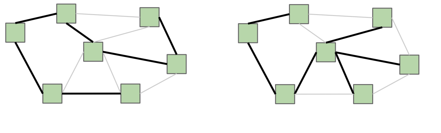
Here’s an example of two different spanning trees on the same graph. Notice how each spanning tree consists of all of the vertices \(V\) in the graph, but exactly \(|V| - 1\) edges while still remaining connected. Because the original graph \(G\) may have many other edges, it’s possible for there to exist multiple spanning trees.

If \(G\) is not a fully-connected graph, then a similar idea is one of a spanning forest, which is a collection of trees, each having a connected component of \(G\), such that there exists a single path between any two vertices in the same connected component.

A minimum spanning tree (MST for short) \(T\) of a weighted undirected graph \(G\) is a spanning tree where the total weight (the sum of all of the weights of the edges) is minimal. That is, no other spanning tree of \(G\) has a smaller total weight.

Consider the graph below.

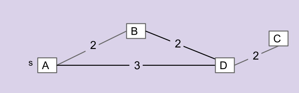
The edges that make up the MST for this graph are \(\overline{AB}\), \(\overline{BD}\), and \(\overline{CD}\). \(\overline{AD}\) is not included in the MST.

MST Algorithms

Before we go into specific algorithms for finding MST’s, let’s talk about the general approach for finding MST’s. To talk about this, we will need to define a few more terms:

• Cut: an assignment of a graph’s vertices into two non-empty sets
• Crossing edge: an edge which connects a vertex from one set to a vertex from the other set

Examples of the above can be found in the following graph below, where the two sets making up the cut are the set of white vertices and the set of gray vertices:

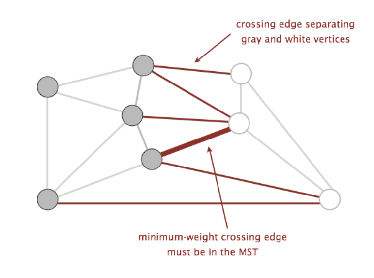
Using these two terms, we can define a new property called the cut property. The cut property states that given any cut of a graph, the minimum weight crossing edge is in the MST. Proving that this is true is slightly out of scope for this course (you will learn more about this in more advanced algorithms classes, such as CS 170), but we will use this property as a backbone for the algorithms we will discuss.

The question is now, what cuts of the graph do we use to find the minimum weight crossing edges to add to our MST? Random cuts may not be the best way to approach this problem, so we’ll go into the following algorithms that each determine cuts in their own way: Prim’s algorithm and Kruskal’s algorithm.

Prim’s Algorithm

Prim’s algorithm is a greedy algorithm that constructs an MST, \(T\), from some graph \(G\) as follows:

1. Create a new graph \(T\), where \(T\) will be the resulting MST.
2. Choose an arbitrary starting vertex in \(G\) and add that vertex to \(T\).
3. Repeatedly add the smallest edge of \(G\) that has one vertex inside \(T\) to \(T\). Let’s call this edge \(e\).
4. Continue until \(T\) has \(V - 1\) edges.

Now, what cuts do we use in this algorithm? We know that at any given point, the two sets of vertices that make up the cut are the following:

• vertices of \(T\)
• vertices of \(G\) that aren’t in \(T\)

Because our algorithm will always add \(e\), the smallest edge of \(G\) that has one vertex inside \(T\) and the other vertex not in \(T\), to the MST \(T\), we will always be adding the minimum edge that crosses the above cut. If the entire tree is constructed in this way, we will have created our MST!

Now, how do we implement this algorithm? We will just need a way to keep track of what \(e\) is at any given time. Because we always care about the minimum, we can use a priority queue!

The priority queue will contain all vertices that are not part of \(T\), and the priority value of a particular vertex \(v\) will be the weight of the shortest edge that connects \(v\) to \(T\). At the beginning of every iteration, we will remove the vertex \(u\) whose connecting edge to \(T\) has the smallest weight, and add the corresponding edge to \(T\). Adding \(u\) to \(T\) will grow our MST, meaning that there will be more edges to consider that have one vertex in \(T\) and the other vertex not in \(T\). For each of these edges \((u, w)\), if this edge has smaller weight than the current edge that would connect \(w\) to \(T\), then we will update \(w\)’s priority value to be the weight of edge \((u, w)\).

Does this procedure sound familiar? Prim’s algorithm actually bears many similarities to Dijkstra’s algorithm, except that Dijkstra’s uses the distance from the start vertex rather than the distance from the MST as the priority values in the priority queue. However, due to Prim’s algorithm’s similarity to Dijkstra’s algorithm, the runtime of Prim’s algorithm will be exactly the same as Dijkstra’s algorithm!

To see a visual demonstration of Prim’s algorithm, see the Prim’s Demo.

Worksheet 2.1 & 2.3: Prim’s Algorithm & Runtime

To get practice running Prim’s algorithm, complete exercise 2.1 on the worksheet. Then, write down the runtime of Prim’s algorithm in 2.3.

Kruskal’s Algorithm

Let’s discuss the second algorithm, Kruskal’s algorithm, another algorithm that can calculate the MST of \(G\). It goes as follows:

1. Create a new graph \(T\) with the same vertices as \(G\), but no edges (yet).
2. Make a list of all the edges in \(G\).
3. Sort the edges from smallest weight to largest weight.
4. Iterate through the edges in sorted order. For each edge \((u, w)\), if \(u\) and \(w\) are not connected by a path in \(T\), add \((u, w)\) to \(T\).

What are the cuts for this algorithm? For Kruskal’s algorithm, the cut will be made by the following sets of vertices:

• vertices of \(T\) connected by any edge
• vertices of \(T\) not connected by any edge

Because Kruskal’s algorithm never adds an edge that connects vertices \(u\) and \(w\) if there is a path that already connects the two, \(T\) is going to be a tree. Additionally, we will be processing the vertices in sorted order, so if we come across an edge that crosses the cut, then we know that that edge will be the minimum weight edge that crosses the cut. Continually building our tree in this way will result in building the MST of the original graph \(G\).

To see a visual demonstration of Kruskal’s algorithm, see the Kruskal’s Demo.

In addition, the USFCA visualization can also be a helpful resource.

The trickier part of Kruskal’s is determining if two vertices \(u\) and \(w\) are already connected. We could do a DFS or BFS starting from \(u\) and seeing if we visit \(w\), though we’d have to do this for each edge. Instead, we can revisit the data structure that specializes in determining if connections exist, the disjoint sets data structure! Each of the vertices of \(G\) will be an item in our data structure. Whenever we add an edge \((u, w)\) to \(T\), we can union the sets that \(u\) and \(w\) belong to. To check if there is already a path connecting \(u\) and \(w\), we can call find on both of them and see if they are part of the same set!

Worksheet 2.2 & 2.3: Kruskal’s Algorithm & Runtime

To get practice running Kruskal’s algorithm, complete exercise 2.2 on the worksheet. Then, write down the runtime (one using DFS/BFS for cycle detection and the other using disjoint sets) of Kruskal’s algorithm in 2.3.

Assume your graph is connected.

Exercise: Prim’s and Kruskal’s Algorithm

Before we implement Prim’s and Kruskal’s algorithm, let’s familiarize ourselves with the graph implementation for this lab.

Graph Representation

Graph.java and Edge.java will define the Graph API we will use for this lab. It’s a bit different from previous labs and so we will spend a little time discussing its implementation. In this lab, our graph will employ vertices represented by integers, and edges represented as an instance of Edge.java. Vertices are numbered starting from 0, so a Graph instance with \(N\) vertices will have vertices numbered from 0 to \(N - 1\). A Graph instance maintains three instance variables:

• neighbors: a HashMap mapping vertices to a set of its neighboring vertices.
• edges: a HashMap mapping vertices to its adjacent edges.
• allEdges: a TreeSet of all the edges present in the current graph.

A Graph instance also has a number of instance methods that may prove useful. Read the documentation to get a better understanding of what each does!

Testing

To test the code that you will write, we have included a directory named inputs, another named outputs, and a few methods that will help generate test graphs.

The inputs directory contains text documents (ending in .in) which can be read in by Graph.java to create a new Graph object. Once this input Graph is created, then you can run one of the MST finding algorithms and compare the output to a Graph whose text document (ending in .out) is contained in the outputs directory.

The syntax for these text documents files is as follows:

# Each line defines a new edge in the graph. The format for each line is
# fromVertex, toVertex, weight
0, 1, 3
1, 2, 2
0, 2, 1

This document creates a graph with three edges. One from vertex 0 to 1 with weight 3, one from 1 to 2 with weight 2, and one from 0 to 2 with weight 1. You may optionally have your text file only add vertices into the graph. This can be done by having each line contain one number representing the vertex you want to add.

# Start of the file.
0
4
2

This creates the graph with vertices 0, 4, and 2. You can define and use your own test inputs by creating a file, placing it into inputs and then reading it in using GraphTest.loadFromText!

Other methods that you may find helpful are Graph.spans, which returns true whether some Graph spans a different inputted Graph, and GraphTest.randomGraph, which generates a random graph with a certain number of vertices, edges, and possible edge weights (note that this method could potentially generate an unconnected graph).

prims

Now, fill in the prims method of the Graph class. You may want to refer back to your code for Dijkstra’s algorithm from lab 17 for inspiration. Keep in mind the different graph representation that we have for this lab.

Hint: Whenever we pop a vertex \(v\) off the fringe, we want to add the corresponding Edge object that connects \(v\) to the MST that we are constructing. This means that we should keep a mapping between vertex number \(i\) and the Edge object with minimum weight that connects vertex \(i\) to the MST. Consider maintaining a map called distFromTree that will keep this mapping between integers (vertex numbers) and Edge objects.

You may assume all input graphs are connected. Make sure to test your code once you’ve completed this method!

kruskals

Now, implement Kruskal’s algorithm using disjoint sets by filling out the method kruskals. For the disjoint set data structure, you should use your disjoint sets implementation, UnionFind.

You may assume all input graphs are connected. Make sure to test your code once you’ve completed this method!

Conclusion

To wrap up, we first learned about an important data structure (disjoint sets) that can help us determine connectivity very quickly. We then learned about a few algorithms, Prim’s and Kruskal’s, that will help us find MST’s. Here are some videos showing both Prim’s algorithm and Kruskal’s algorithm. These are two very different algorithms, so make sure to take note of the visual difference in running these algorithms!

Deliverables

To receive credit for this lab:

• Turn in the completed worksheet to your TA at the end of lab.
• Complete the implementation of UnionFind.java
• Complete the prims method.
• Complete the kruskals method.