Introduction

We have already seen a few implementations of the Set ADT, and in this lab we will see a slightly different approach to this ADT. Today we will learn about disjoint sets, which we can use in the tomorrow’s lab to implement some minimum spanning tree algorithms.

As usual, pull the files from the skeleton and make a new IntelliJ project.

Disjoint Sets

Suppose we have a collection of companies that have gone under mergers or acquisitions. We want to develop a data structure that allows us to determine if any two companies are in the same conglomerate. For example, if company X and company Y were originally independent but Y acquired X, we want to be able to represent this new connection in our data structure. How would we do this? One way we can do this is by using the disjoint sets data structure.

The disjoint sets data structure represents a collection of sets that are disjoint, meaning that any item in this data structure is found in no more than one set. When discussing this data structure, we often limit ourselves to two operations, union and find, which is also why this data structure is sometimes called the union-find data structure. We will be using the two interchangeably for the remainder of this lab.

The union operation will combine two sets into one set. The find operation will take in an item, and tell us which set that item belongs to. With this data structure, we will be able to keep track of the acquisitions and mergers that occur!

Let’s run through an example of how we can represent our problem using disjoint sets with the following companies:

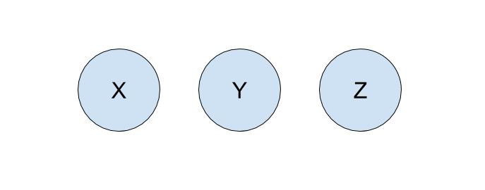
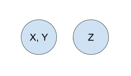
To start off, each company is in its own set with only itself and a call to find(X) will return \(X\) (and similarly for all the other companies). If \(Y\) acquired \(X\), we will make a call to union(X, Y) to represent that the two companies should now be linked. As a result, a call to find(X) will now return \(Y\), showing that \(X\) is now a part of \(Y\). The unioned result is shown below.

Quick Find

For the rest of the lab, we will work with non-negative integers as the items in our disjoint sets. If you wanted to have a disjoint set of something that did not correspond to a set of integers, you could generalize this data structure by maintaining some sort of mapping between whatever the objects are and the set of integers contained within the disjoint set data structure.

In order to implement disjoint sets, we need to know the following:

• What items are in each set
• Which set each item belongs to

One implementation we can do involves keeping an array that details just that. In our array, the index will represent the item (hence non-negative integers) and the value at that index will represent which set that item belongs to. For example, if our set looked like this,

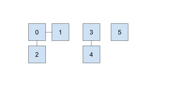
then we could represent the connections like this:

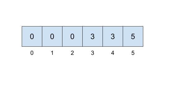
Here, we will be choosing the smallest number of the set to represent the face of the set, which is why the set numbers are 0, 3, and 5.

This approach uses the quick-find algorithm, prioritizing the runtime of the find operation but making the union operations slow. But, how fast is the find operation in the worst case, and how slow is the union operation in the worst case? Discuss with your partner, then check your answers below. Hint: Think about the example above, and try out some find and union operations yourself!

Answer below (highlight to reveal):

1. Worst-case runtime for quick-find data structure's find with $N$ items: $\Theta(1)$
2. Worst-case runtime for quick-find data structure's union with $N$ items: $\Theta(N)$

Quick Union

Suppose we prioritize making the union operation fast instead. One way we can do that is that instead of representing each set as we did above, we will think about each set as a tree.

This tree will have the following qualities:

• the nodes will be the items in our set,
• each node only needs a reference to its parent rather than a direct reference to the face of the set, and
• the top of each tree (we refer to this top as the “root” of the tree) will be the face of the set it represents.

In the example from the beginning of lab, \(Y\) would be the face of the set represented by \(X\) and \(Y\), so \(Y\) would be the root of the tree containing \(X\) and \(Y\).

How do we modify our data structure from above to make this quick union? We will just need to replace the set references with parent references! The indices of the array will still correspond to the item itself, but we will put the parent references inside the array instead of direct set references. If an item does not have a parent, that means this item is the face of the set and we will instead record the size of the set. In order to distinguish the size from parent references, we will record the size, \(s\), of the set as \(-s\) inside of our array. The reason we store the size will not be very clear for this iteration of our data structure, but will allow us some future optimizations!

When we union(u, v), we will find the set that each of the values belong to (the roots of their respective trees), and make one the child of the other. If u and v are both the face of their respective sets and in turn the roots of their own tree, union(u, v) is a fast \(\Theta(1)\) operation because we just need to make the root of one set connect to the root of the other set!

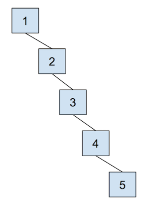
The cost of a quick union, however, is that find can now be slow. In order to find which set an item is in, we must jump through all the parent references and travel to the root of the tree, which is \(\Theta(N)\) in the worst case. Here’s an example of a tree that would lead to the worst case runtime, which we again refer to as “spindly”:

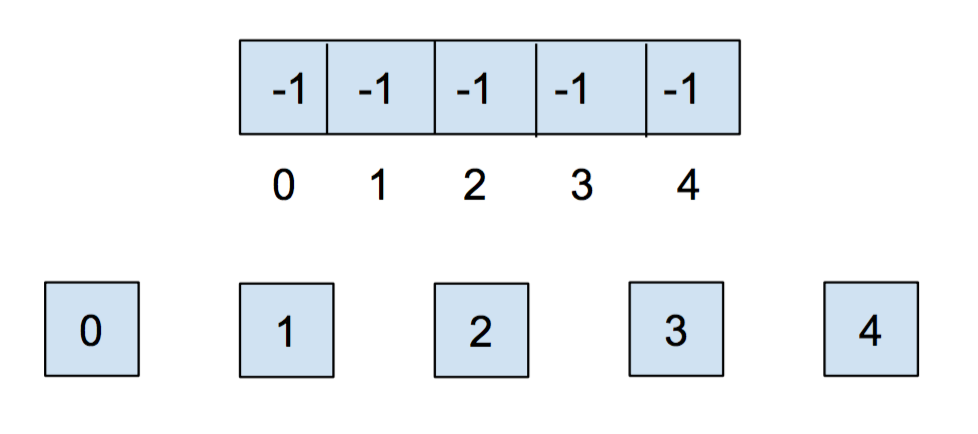
In addition, union-ing two leaves could lead to the same worst case runtime as find because we would have to first find the sets that each of the leaves belong to before completing union operation. We will soon see some optimizations that we can do in order to make this runtime faster, but let’s go through an example of this quick union data structure first. The array representation of the data structure is shown first, followed by the abstract tree representation of the data structure.

Initially, each item is in its own set, so we will initialize all of the elements in the array to -1.

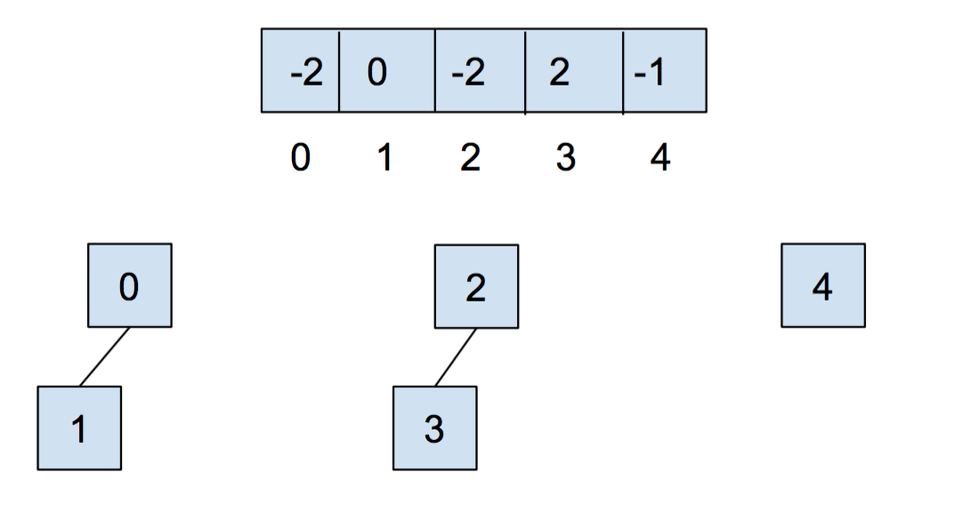
After we call union(0,1) and union(2,3), our array and our abstract representation look as below:

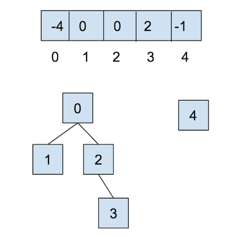
After calling union(0,2), they look like:

Now, let’s combat the shortcomings of this data structure with the following optimizations.

Weighted Quick Union

The first optimization that we will do for our quick union data structure is called “union by size”. This will be done in order to keep the trees as shallow as possible and avoid the spindly trees that result in the worst-case runtimes. When we union two trees, we will make the smaller tree (the tree with less nodes) a subtree of the larger one, breaking ties arbitrarily. We call this weighted quick union.

Because we are now using “union by size”, the maximum depth of any item will be in \(O(\log N)\), where \(N\) is the number of items stored in the data structure. This is a great improvement over the linear time runtime of the unoptimized quick union. Some brief intuition for this depth is because the depth of any element \(x\) only increases when the tree \(T_1\) that contains \(x\) is placed below another tree \(T_2\). When that happens, the size of the resulting tree will be at least double the size of \(T_1\) because \(size(T_2) \ge size(T_1)\). The tree that contains only \(x\) can double its size at most \(\log N\) times until we have reached a total of \(N\) items.

Discussion: Weighted Quick Union vs Heighted Quick Union

Define a fully connected DisjointSets object as one in which connected returns true for any arguments, due to prior calls to union.

We have not directly discussed connected yet, but you think about how this could be implemented. How could we use the find operation to check if two different elements are part of the same set.

Suppose we have a fully connected DisjointSets object with 6 items. Give the best and worst case height for the two implementations below. We will define height as the number of links from the root to the deepest leaf, so a tree with 1 element has a height of 0.

Assume HeightedQuickUnion is like WeightedQuickUnion, except uses height instead of weight to determine which subtree is the new root. Hint: For each of these try drawing out a few disjoint set trees and think about the different possible sequences of union operations that will result in the maximum height vs. the minimum height tree.

1. What is the best-case height for a WeightedQuickUnion containing 6 items?
2. What is the worst-case height for a WeightedQuickUnion containing 6 items?
3. What is the best-case height for a HeightedQuickUnion containing 6 items?
4. What is the worst-case height for a HeightedQuickUnion containing 6 items?

Answer below (highlight to reveal):

1. 1
2. 2
3. 1
4. 2

Path Compression

Even though we have made a speedup by using a weighted quick union data structure, there is still yet another optimization that we can do! What would happen if we had a tall tree and called find repeatedly on the deepest leaf? Each time, we would have to traverse the tree from the leaf to the root.

A clever optimization is to move the leaf up the tree so it becomes a direct child of the root. That way, the next time you call find on that leaf, it will run much more quickly. An even more clever idea is that we could do the same thing to every node that is on the path from the leaf to the root, connecting each node to the root as we traverse up the tree. This optimization is called path compression. Once you find an item, path compression will make finding it (and all the nodes on the path to the root) in the future faster.

The runtime for any combination of \(f\) find and \(u\) union operations takes \(\Theta(u + f \alpha(f+u,u))\) time, where \(\alpha\) is an extremely slowly-growing function called the inverse Ackermann function. And by “extremely slowly-growing”, we mean it grows so slowly that for any practical input that you will ever use, the inverse Ackermann function will never be larger than 4. That means for any practical purpose, a weighted quick union data structure with path compression has find operations that take constant time on average!

It is important to note that even though this operation can be considered constant time for all practically sized inputs, we should not describe this whole data structure as constant time. We could say something like, it will be constant for all inputs smaller than some incredibly large size. Without that qualification we should still describe it by using the inverse Ackermann function.

You can visit this link here to play around with disjoint sets.

Exercise: UnionFind

We will now implement our own disjoint sets data structure. When you open up UnionFind.java, you will see that it has a number of method headers with empty implementations.

Read the documentation to get an understanding of what methods need to be filled out. Remember to implement both optimizations discussed above, and take note of the tie-breaking scheme that is described in the comments of some of the methods. This scheme is done for autograding purposes and is chosen arbitrarily. In addition, remember to ensure that the inputs to your functions are within bounds, and should otherwise throw an IllegalArgumentException.

Discussion: UnionFind

Our UnionFind uses only non-negative values as the items in our set.

How can we use the data structure that we created above to keep track of different values, such as all integers or companies undergoing mergers and acquisitions? Discuss with your partner.

Recap

Dynamic Connectivity Problem

The ultimate goal of this lab was to develop a data type that support the following operations on \(N\) objects:

• connect(int p, int q) (called union in our optional textbook)
• isConnected(int p, int q) (called connected in our optional textbook)

We do not care about finding the actual path between p and q. We care only about their connectedness. A third operation we can support is very closely related to connected:

• find(int p): The find method is defined so that find(p) == find(q) if and only if connected(p, q). We did not use this in class.

Connectedness is an equivalence relation

Saying that two objects are connected is the same as saying they are in an equivalence class. This is just fancy math talk for saying “every object is in exactly one bucket, and we want to know if two objects are in the same bucket”. When you connect two objects, you’re basically just pouring everything from one bucket into another.

Quick find

This is the most natural solution, where each object is given an explicit number. Uses an array id of length \(N\), where id[i] is the bucket number of object i (which is returned by find(i)). To connect two objects p and q, we set every object in p’s bucket to have q’s number.

• connect: May require many changes to id. Takes \(\Theta(N)\) time, as the algorithm must iterate over the entire array.
• isConnected (and find): take constant time.

Performing \(M\) operations takes \(\Theta(MN)\) time in the worst case. If \(M\) is proportional to \(N\), this results in a \(\Theta(N^2)\) runtime.

Quick union

An alternate approach is to change the meaning of our id array. In this strategy, id[i] is the parent object of object i. An object can be its own parent. The find method climbs the ladder of parents until it reaches the root (an object whose parent is itself). To connect p and q, we set the root of p to point to the root of q.

• connect: Requires only one change to id, but also requires root finding (worst case \(\Theta(N)\) time).
• isConnected (and find): Requires root finding (worst case \(\Theta(N)\) time).

Performing \(M\) operations takes \(\Theta(NM)\) time in the worst case. Again, this results in quadratic behavior if \(M\) is proprtional to \(N\).

Weighted quick union

Rather than connect(p, q) making the root of p point to the root of q, we instead make the root of the smaller tree point to the root of the larger one. The tree’s size is the number of nodes, not the height of the tree. Results in tree heights of \(\log N\).

• connect: Requires only one change to id, but also requires root finding (worst case \(\log N\) time).
• isConnected (and find): Requires root finding (worst case \(\log N\) time).

Warning: if the two trees have the same size, the book code has the opposite convention as quick union and sets the root of the second tree to point to the root of the first tree. This isn’t terribly important (you won’t be tested on trivial details like these).

Weighted quick union with path compression

When find is called, every node along the way is made to point at the root. Results in nearly flat trees. Making \(M\) calls to union and find with \(N\) objects results in no more than \(O(M \log^* N)\) array accesses, not counting the creation of the arrays. For any reasonable values of \(N\) in this universe that we inhabit, \(\log^* N\) is at most 5.

Deliverables

To receive credit for this lab:

• Complete the implementation of UnionFind.java