
Introduction
As usual, pull the files from the skeleton and make a new IntelliJ project.
In previous labs, we have seen various types of graphs, including weighted, undirected graphs, as well as algorithms that can be performed on them. In this lab, we will be introducing a few algorithms which can be used to find a minimum spanning tree.
Minimum Spanning Tree
Consider an undirected graph \(G = (V,E)\) comprising of a set of vertices, \(V\), and a set of edges, \(E\). Let’s break down the term, minimum spanning tree.
A tree is an acyclic (has no cycles) and connected graph. If it has \(N\) vertices, then it must have exactly \(N - 1\) edges in order to satisfy these properties. A tree can be as small as just a single node in a large graph.
A spanning tree further requires not just any small tree in the graph, but one which spans all the vertices in the graph. Formally, a spanning tree \(T = (V, F)\) of \(G\) is a tree that contains all of the vertices of \(V\) of the graph \(G\), and a subset of its edges: \(F \subseteq E\), where \(|F| = |V| - 1\) edges from \(G\).
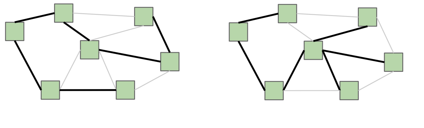
Here’s an example of two different spanning trees on the same graph. Notice how each spanning tree consists of all of the vertices \(V\) in the graph, but exactly \(|V| - 1\) edges while still remaining connected. Because the original graph \(G\) may have many other edges, it’s possible for there to exist multiple spanning trees.
If \(G\) is not a fully-connected graph, then a similar idea is one of a spanning forest, which is a collection of trees, each having a connected component of \(G\), such that there exists a single path between any two vertices in the same connected component.
A minimum spanning tree (MST for short) \(T\) of a weighted undirected graph \(G\) is a spanning tree where the total weight (the sum of all of the weights of the edges) is minimal. That is, no other spanning tree of \(G\) has a smaller total weight.
Consider the graph below. Which edge is not in the MST of this graph? Discuss with your partner.
\[\overline{AB}, \overline{AD}, \overline{BD}, \overline{DC}\]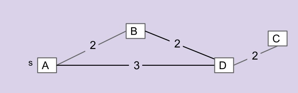
MST Algorithms
Before we go into specific algorithms for finding MST’s, let’s talk about the general approach for finding MST’s. To talk about this, we will need to define a few more terms:
- Cut: an assignment of a graph’s vertices into two non-empty sets
- Crossing edge: an edge which connects a vertex from one set to a vertex from the other set
Examples of the above can be found in the following graph below, where the two sets making up the cut are the set of white vertices and the set of gray vertices:
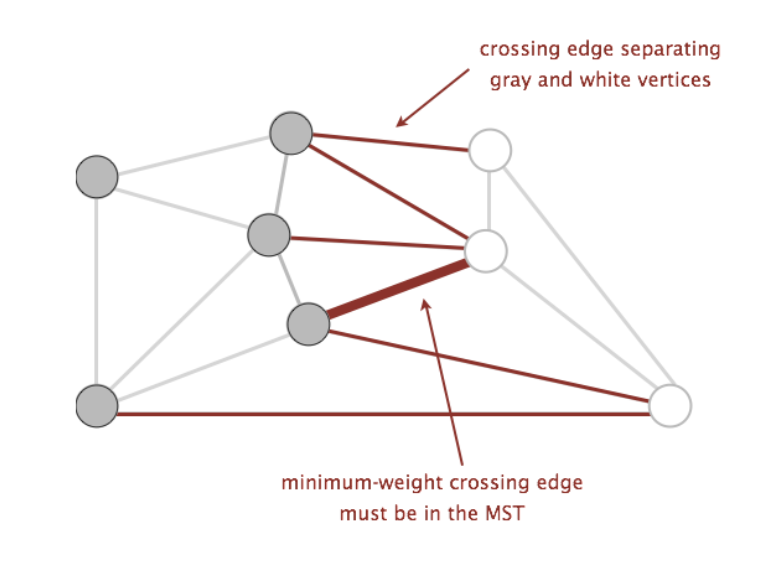
Using these two terms, we can define a new property called the cut property. The cut property states that given any cut of a graph, the minimum weight crossing edge is some valid MST (as there can be multiple). Proving that this is true is slightly out of scope for this course (you will learn more about this in more advanced algorithms classes, such as CS 170), but we will use this property as a backbone for the algorithms we will discuss.
The question is now, what cuts of the graph do we use to find the minimum weight crossing edges to add to our MST? Random cuts may not be the best way to approach this problem, so we’ll go into the following algorithms that each determine cuts in their own way: Prim’s algorithm and Kruskal’s algorithm.
Prim’s Algorithm
Prim’s algorithm is a greedy algorithm that constructs an MST, \(T\), from some graph \(G\) as follows:
- Create a new graph \(T\), where \(T\) will be the resulting MST.
- Choose an arbitrary starting vertex in \(G\) and add that vertex to \(T\).
- Repeatedly add the smallest edge of \(G\) that has one vertex inside \(T\) to \(T\). Let’s call this edge \(e\).
- Continue until \(T\) has \(V - 1\) edges.
Now, what cuts do we use in this algorithm? We know that at any given point, the two sets of vertices that make up the cut are the following:
- vertices of \(T\)
- vertices of \(G\) that aren’t in \(T\)
Because our algorithm will always add \(e\), the smallest edge of \(G\) that has one vertex inside \(T\) and the other vertex not in \(T\), to the MST \(T\), we will always be adding the minimum edge that crosses the above cut. If the entire tree is constructed in this way, we will have created our MST!
Now, how do we implement this algorithm? We will just need a way to keep track of what \(e\) is at any given time. Because we always care about the minimum, we can use a priority queue!
The priority queue will contain all vertices that are not part of \(T\), and the priority value of a particular vertex \(v\) will be the weight of the shortest edge that connects \(v\) to \(T\). At the beginning of every iteration, we will remove the vertex \(u\) whose connecting edge to \(T\) has the smallest weight, and add the corresponding edge to \(T\). Adding \(u\) to \(T\) will grow our MST, meaning that there will be more edges to consider that have one vertex in \(T\) and the other vertex not in \(T\). For each of these edges \((u, w)\), if this edge has smaller weight than the current edge that would connect \(w\) to \(T\), then we will update \(w\)’s priority value to be the weight of edge \((u, w)\).
Does this procedure sound familiar? Prim’s algorithm actually bears many similarities to Dijkstra’s algorithm, except that Dijkstra’s uses the distance from the start vertex rather than the distance from the MST as the priority values in the priority queue. However, due to Prim’s algorithm’s similarity to Dijkstra’s algorithm, the runtime of Prim’s algorithm will be exactly the same as Dijkstra’s algorithm!
To see a visual demonstration of Prim’s algorithm, see the Prim’s Demo.
Exercise: Prim’s Algorithm
Before we implement Prim’s algorithm, let’s familiarize ourselves with the graph implementation for this lab.
Graph Representation
Graph.java and Edge.java will define the Graph API we will use for this lab. It’s a bit different from previous labs and so we will spend a little time discussing its implementation. In this lab, our graph will employ vertices represented by integers, and edges represented as an instance of Edge.java. Vertices are numbered starting from 0, so a Graph instance with \(N\) vertices will have vertices numbered from 0 to \(N - 1\). A Graph instance maintains three instance variables:
neighbors: aHashMapmapping vertices to a set of its neighboring vertices.edges: aHashMapmapping vertices to its adjacent edges.allEdges: aTreeSetof all the edges present in the current graph.
A Graph instance also has a number of instance methods that may prove useful. Read the documentation to get a better understanding of what each does!
prims
Now, fill in the prims method of the Graph class. You may want to refer back to your code for Dijkstra’s algorithm from lab 19 for inspiration. Keep in mind the different graph representation that we have for this lab.
Hint: Whenever we pop a vertex \(v\) off the fringe, we want to add the corresponding Edge object that connects \(v\) to the MST that we are constructing. This means that we should keep a mapping between vertex number \(i\) and the Edge object with minimum weight that connects vertex \(i\) to the MST. Consider maintaining a map called distFromTree that will keep this mapping between integers (vertex numbers) and Edge objects.
Testing
To test the code that you have just written, we have included a directory named inputs and a few methods that will help generate test graphs. The inputs directory contains text documents which can be read in by Graph.java to create a new graph. The syntax for the input files is as follows:
# Each line defines a new edge in the graph. The format for each line is
# fromVertex, toVertex, weight
0, 1, 3
1, 2, 2
0, 2, 1
This document creates a graph with three edges. One from vertex 0 to 1 with weight 3, one from 1 to 2 with weight 2, and one from 0 to 2 with weight 1. You may optionally have your text file only add vertices into the graph. This can be done by having each line contain one number representing the vertex you want to add.
# Start of the file.
0
4
2
This creates the graph with vertices 0, 4, and 2. You can define and use your own test inputs by creating a file, placing it into inputs and then reading it in using Graph.loadFromText!
Kruskal’s Algorithm
Let’s discuss the second algorithm, Kruskal’s algorithm, another algorithm that can calculate the MST of \(G\). It goes as follows:
- Create a new graph \(T\) with the same vertices as \(G\), but no edges (yet).
- Make a list of all the edges in \(G\).
- Sort the edges from smallest weight to largest weight.
- Iterate through the edges in sorted order. For each edge \((u, w)\), if \(u\) and \(w\) are not connected by a path in \(T\), add \((u, w)\) to \(T\).
Optional Introduction Video
What are the cuts for this algorithm? For Kruskal’s algorithm, the cut will be made by the following sets of vertices:
- vertices of \(T\) connected by any edge
- vertices of \(T\) not connected by any edge
Because Kruskal’s algorithm never adds an edge that connects vertices \(u\) and \(w\) if there is a path that already connects the two, \(T\) is going to be a tree. Additionally, we will be processing the vertices in sorted order, so if we come across an edge that crosses the cut, then we know that that edge will be the minimum weight edge that crosses the cut. Continually building our tree in this way will result in building the MST of the original graph \(G\).
Both Prim’s and Kruskal’s are greedy algorithms, but in different ways. Discuss the commonalities and important distinctions between the two algorithms with your partner.
Exercise: Kruskal’s Runtime
Exercise 1: Using a Traversal
How about the runtime of Kruskal’s algorithm? As we will see in future labs, sorting \(|E|\) edges will take \(O(|E| \lg |E|)\) time (just accept this fact for now!). The trickier part of Kruskal’s is determining if two vertices \(u\) and \(w\) are already connected. We could do a DFS or BFS starting from \(u\) and seeing if we visit \(w\), though we’d have to do this for each edge. What would be the resulting worst case runtime for Kruskal’s algorithm if it were implemented in this way?
Discuss this with your partner and then highlight the next line to verify your work.
Theta(EV).
Exercise 2: Using Disjoint Sets
Instead, let’s revisit the data structure that specializes in determining if connections exist, the disjoint sets data structure. Each of the vertices of \(G\) will be an item in our data structure. Whenever we add an edge \((u, w)\) to \(T\), we can union the sets that \(u\) and \(w\) belong to. To check if there is already a path connecting \(u\) and \(w\), we can call find on both of them and see if they are part of the same set. Using this data structure, what is the runtime of Kruskal’s algorithm? (Note, this assumes that graph creation is in constant time. If it is not, then we must take that into consideration as well.)
Discuss this with your partner and then highlight the next line to verify your work.
Theta(E log(E)).
To see a visual demonstration of Kruskal’s algorithm, see the Kruskal’s Demo.
In addition, the USFCA visualization can also be a helpful resource.
Exercise: Kruskal’s Algorithm
Now, implement Kruskal’s algorithm using disjoint sets by filling out the method kruskals. You may also use techniques discussed in the Testing section above to test your implementation of Kruskal’s algorithm. For the disjoint set data structure, you may import the WeightedQuickUnionUF class but you are strongly encouraged to use your implementation from lab20.
Conclusion
To wrap up, here are some videos showing both Prim’s algorithm and Kruskal’s algorithm. These are two very different algorithms, so make sure to take note of the visual difference in running these algorithms!
Deliverables
As always, ensure you added, committed, taged, pushed, and push –tag from your partnership repo.
To get credit for this lab:
- Complete the
primsmethod. - Complete the
kruskalsmethod.