FAQ #

Each assignment will have an FAQ linked at the top. You can also access it by adding “/faq” to the end of the URL. The FAQ for Lab 14 is located here.

Before You Begin #

As usual, pull the Lab 15 files from the skeleton and open them in in IntelliJ.

Learning Goals #

In this lab, we will:

• Describe balanced search trees and compare them to regular binary search trees;
• Describe the properties and algorithms for 2-3 trees
• Connect 2-3 tree concepts to red-black trees
• Implement a left-leaning red-black tree

Introduction #

Over the past few labs, we have analyzed the performance of algorithms for access and insertion into binary search trees. However, our analyses often made the assumption that the trees were balanced.

Informally, a tree being “balanced” means that the paths from root to leaves are all roughly the same length. Any algorithm that looks once at each level of the tree – such as searching for a value in a binary search tree – only looks at the number of layers. As we discovered in the previous lab, the smallest number of layers we can have is logarithmic with respect to the of nodes. Balanced trees prevent the worst case scenarios where we have “spindly”, unbalanced trees, which may have a linear number of layers.

In the binary search tree we saw last lab, this balancing doesn’t happen automatically. We’ve also seen how to insert items into a binary search tree to produce this worst-case linear time behavior.

There are two approaches we can take to make trees balanced:

Incremental balancing

At each insertion or deletion we do a bit of work to keep the tree balanced.

All-at-once balancing

We don’t do anything to keep the tree balanced until it gets too lopsided, then we completely rebalance the tree.

We will only look at trees that perform incremental balancing.

2-3 Trees #

Throughout this lab, we will use the term “key” to define a value that is stored in the tree (previously element, a much longer word).

In a binary search tree, each tree node contains exactly one key. To avoid the worst-case scenario, let’s change this up. Instead of storing a single key per node, we will store multple keys per node. Specifically, we’ll allow nodes to contain two elements! This is the 2-3 tree.

A 2-3 tree is a tree in which each non-leaf node has either 2 or 3 children. Additionally, any non-leaf node must have one more child than key. That means that a node with 1 key must have 2 children, and a node with 2 keys must have 3 children.

We refer to a node with N children as an “N-node”, so a node with 1 key and 2 children would be called a 2-node, and a node with 2 keys and 3 children would be called a 3-node.

Additionally, there are ordering invariants similar to the binary search tree. Nodes with 1 key and 2 children have the same invariant as a binary search tree, where keys in the left subtree must all be smaller; and keys in the right subtree must all be greater.

We can extend this to 3-nodes as well. First, the left key must be smaller than the right key. Nodes in the left subtree must be less than the smaller key; nodes in the middle subtree must be between the two keys; and nodes in the right subtree must be greater than the larger key. node.

As in binary search trees, these ordering invariants must recursively hold. Additionally, just like the previous lab, we won’t consider equal keys at all.

Here’s an example of a 2-3 tree:

Exercise: Searching a 2-3 Tree #

We can take advantage of the ordering property to construct a search algorithm similar to the search algorithm for binary search trees. Assume that within a node, we check keys from left to right.

Discuss the following with your partner, based on the tree above:

1. What is the order in which we check keys when we search for 7 (a key in the tree)?
2. What is the order in which we check keys when we search for 13 (a key not in the tree)?

Answers (click to view):

1. Check 5, see that it’s greater. Check 9, see that it’s smaller, explore to the middle child. Check 7, see that we’ve found the key.
2. Check 5, see that it’s greater. Check 9, see that it’s greater, explore to the right child. Check 10, see that it’s greater. Check 12, see that it’s greater. No more children, so conclude that it’s not in the tree.

Insertion into a 2-3 Tree #

Although searching in a 2-3 tree is like searching in a BST, inserting a new item is a little different.

Similar to a BST, we always insert the new key in a leaf node. We must find the correct place for the key that we insert to go by traversing down the tree, and then insert the new key into the appropriate place in the existing leaf. However, unlike in a BST, we can “stuff” more keys into the nodes in a 2-3 tree.

Basic Insertion #

Suppose we have the 2-3 tree from above:

If we were to insert 8 into the tree, we first traverse down the tree until we find the proper leaf node to insert it into: the 7 node. Since 8 is larger than 7, we insert it to the right of the 7.

Push-Up Insertion #

However, what if the leaf node we choose to insert into already has 2 keys? Even though we’d like to put the new item there, it won’t fit because nodes can have no more than 2 keys. What should we do?

Consider the following 2-3 tree:

Let’s try to insert 4. We see that it needs to go into the leaf node to the left with keys [1, 3]. We start by temporarily violating the 3-key limitation, and “overstuffing” this node so that it has keys [1, 3, 4].

We need to “split” this node with 3 keys, so that all nodes continue to have 1 or 2 keys. One way to do that could be to create a subtree, by moving the middle node “up”, and splitting the remaining nodes.

However, this makes some of the leaves (1 and 4) be further from the root than other leaves (7 and 9). We want to keep our tree as balanced as possible, so we want to keep our leaves at the same height. To fix this, instead of keeping the middle key separate, we “push it up” to the parent node:

The tree invariants now hold, so we’re done! Note that the other two keys in the overstuffed node (1 and 4) have become separate children of the newly expanded node with keys 3 and 5.

Push-Up Insertion… Again #

You may have noticed a problem in the previous section. What if this push-up causes the parent node to have too many keys? When the parent node has too many keys, we need to push up and split again – which may cause another overstuffing, and so on.

Let’s insert 8 into the tree we finished with last time:

Since we have an overstuffed node, we need to split and push up:

When we create an overstuffed node that temporarily has 3 keys, it has 4 children, since all nodes have 1 more child than key.

When we reach the root node, we don’t have a parent node to push up into. Instead, we push up the middle node (as usual), and create a new layer. This does not cause any of the leaves to be at different heights from the root. We’re making a new root, and pushing down all leaves equally!

Wait, what happened to the 4 children from the split node – why did they go there? Remember the binary search tree-like invariant. After we pull up 5 and have 3 and 8 be split into separate children, we must maintain the ordering invariant. The subtree rooted at 4 could contain any keys “between 3 and 5”. To keep that true, we put 4’s subtree in the new tree where it could still contain any keys between 3 and 5 – to the left of 5, then to the right of 3.

Push-Up Insertion Summary #

Here’s a summary of different cases you might encounter when performing push-up insertion. Each of these cases can be explained by upholding the binary search invariant.

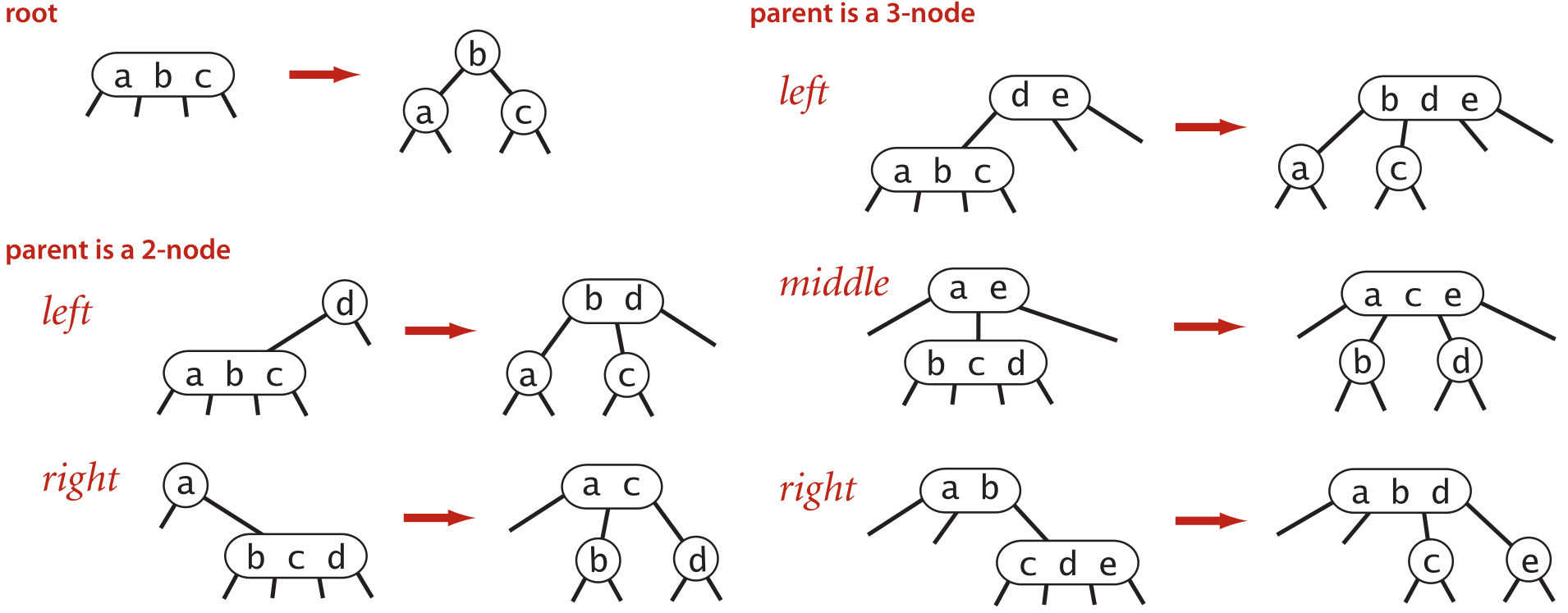
Diagram from Sedgewick’s Algorithms, 4th ed.

Exercise: Growing a 2-3 Tree #

1. Insert 10, 11, 12, and 13 in order into the final 2-3 tree above. Then, compare your answer with your partner’s.

2. Suppose the keys 1, 2, 3, 4, 5, 6, 7, 8, 9, and 10 are inserted sequentially into an initially empty 2-3 tree. Which insertion causes the second split to take place?

   Try to add these keys to an empty tree, and discuss your result with your partner.

If you want to check your work, consider using this visualization tool from the University of San Francisco. Make sure to set the degree of the tree appropriately. They have a few more interesting visualizations on their site if you want to use as a resource at a later point.

To get the starting tree for (1), a sequence of insertions is 3, 5, 7, 1, 9, 4, 8.

Discuss: 2-3 Tree Balancing #

With the insertion procedure given above, why are 2-3 trees self-balancing? Can a leaf ever be further from the root than another? Discuss with your partner.

Left-Leaning Red-Black Trees #

We saw that 2-3 trees are balanced, guaranteeing that a path from the root to any leaf is \(O(\log N)\). However, 2-3 trees are notoriously difficult and cumbersome to code, with numerous corner cases for common operations. They are commonly used and have significant (out-of-scope) benefits, but they also have drawbacks.

We turn our attention to a related data structure, the red-black tree (in fact, the tree behind Java’s TreeSet and TreeMap). A red-black tree at its core is just a binary search tree, but there are a few additional invariants related to “coloring” each node red or black. This “coloring” creates a mapping between 2-3 trees and red-black trees! In particular, every 2-3 tree corresponds to exactly one red-black tree, and vice-versa.

The consequence is quite astounding: red-black trees maintain the balance of 2-3 trees while inheriting all normal binary search tree operations (a red-black tree is a binary search tree after all) with additional housekeeping. These qualities, self-balancing combined with ease of binary search operations, is why Java’s TreeMap and TreeSet are implemented as red-black trees!

We will concern ourselves with a specific subset of red-black trees: left-leaning red-black trees, or LLRB trees.

2-3 Trees ↔ LLRB Trees #

Notice that a 2-3 tree can have 1 or 2 elements per node, with 2 or 3 children respectively. We would like to use a standard binary tree to be able to represent a 2-3 tree. It is straightforward to represent nodes with 1 key – they are regular nodes, with one key and two children. However, how do we represent nodes with two keys?

We split the two keys into two nodes, and color them:

Note the location of the child subtrees. Here, we’ve colored a red, to indicate that it is in the same 2-3 tree node as its parent. We color all other nodes black to indicate that they are in a different 2-3 tree node from their parent.

In this way, we also see that each 2-3 tree node corresponds to exactly one black node (and vice-versa).

Note that a could have been on top, with b being a child on the right. This is also technically valid! However, to simplify the cases we later consider, we always put the single red child on the left. This is what makes these trees left-leaning.

Here’s a full 2-3 tree translated into the corresponding LLRB tree:

LLRB Tree Properties #

We can now specify some properties of LLRB trees that allow us to define them independently. In particular, we use the one-to-one mapping between valid LLRB trees and 2-3 trees to derive some of these properties.

The root node must be colored black.

Our interpretation of red nodes is that they are in the same 2-3 node as their parent. The root node has no parent, so it cannot be red.

If a node has one red child, it must be on the left.

This makes the tree left-leaning.

No node can have two red children.

If a node has two red children, then both children are in the same 2-3 node as the parent. This means that the corresponding 2-3 node contains 3 keys, which is not allowed.

No red node can have a red parent; or every red node’s parent is black.

If a red node has a red parent, then both the red child and red parent are in the same 2-3 node as the red parent’s parent. This means that the corresponding 2-3 node contains 3 keys, which is not allowed.

In a balanced LLRB tree, every path to a leaf goes through the same number of black nodes.

In a balanced 2-3 tree, every leaf node is the same distance from the root. We also know that every black node in an LLRB tree corresponds to exactly one node in the equivalent 2-3 tree. Therefore, every leaf node in an LLRB tree is the same number of black nodes from the root, just as every leaf node in a 2-3 tree is the same distance from the root.

Discussion: LLRB Tree Properties #

Given the height of a 2-3 tree, what is the maximum height of the corresponding LLRB tree? Discuss with your partner.

Then, discuss with your partner about which of the following binary search tree operations we can use on red-black trees without any modification.

1. Insertion
2. Deletion
3. Search (is k in the tree?)
4. Range Queries (return all items between a and b)

Answers (click to view):

The tallest LLRB tree that we can get from a 2-3 tree is by stacking 3-nodes, which contain a black node on top of a red node. The height of the LLRB tree is therefore double the height of the corresponding 2-3 tree.

We can perform searches and range queries just like for binary search trees, since these don’t modify the tree structure. However, we must change our insertion and deletion algorithms to uphold the invariants we just discussed.

Exercise: Constructor #

Read the code in RedBlackTree.java and 23Tree.java.

Then, in RedBlackTree.java, implement buildRedBlackTree which returns the root node of the red-black tree which has a one-to-one mapping to the given 2-3 tree. For a 2-3 tree node with 2 elements in a node, you must create a left-leaning red child to pass the autograder tests.

If you’re stuck, refer to the example conversions shown above to help you write this method!

Some further tips for writing this method if you are stuck:

• You should be filling in the two cases which correspond to a 2-node and a 3-node. For a 2-node, you should need to make one new RBTreeNode object. For a 3-node, you should need to make two new RBTreeNode objects.
• You should rely on the getItemAt and getChildAt methods from the Node class which will return the appropriate items and children Nodes.
• Your code should involve the same number of recursive calls to buildRedBlackTree as the number of children in the Node you are translating, e.g. two recursive calls for a 2-node and three recursive nodes for a 3-node.
• For both cases you should only make one of the RBTreeNodes be a black node. For the cases where you have more than one RBTreeNode make sure that you are returning the black node.

Inserting Into LLRB Trees #

Insertion into LLRB trees starts off with the regular binary search tree insertion algorithm, where we search to find the appropriate leaf location. However, once we’ve placed the node, this can can break the red-black tree invariants, so we need additional operations that can “restore” the red-black tree properties. We know that there is a one-to-one correspondence of valid red-black trees to 2-3 trees. Let’s use this correspondence to try to derive these operations.

Throughout:

• Our newly added node will have the key x. We will use letters, such as a and b to represent the other relevant values. They are ordered among each other (a < b), but assume that x’s value is whatever it needs to be to be in the right location.
• Our newly added node will be red. When we add to a 2-3 tree, we always stuff leaf before splitting – therefore, our new node is in the same 2-3 node as its arent LLRB node.

Case: Only Child of a Black Node #

Since a black node corresponds to a 2-node with 1 key, there are two possible places that the new red node could end up, depending on its value:

This case is fine, since the red child is on the left. No further action is needed.

However, what if x > a? Then,

This is violation of the invariant that a single red child is on the left. It seems like we want these nodes to be “turned” the other way, with x as the parent and a as the red child – moving a and x to the left. To do this, we use the operation “rotate left” on the parent node a.

Here’s a few things to notice about this “rotation”:

• The root of the subtree has changed from a to b.
• a and b have moved to the “left”.
• The two nodes swap colors so that the new root is the same color as the old root.
• The reorganized subtree still satisfies the binary search property.

Applying the rotation to the violation above by rotating left on a, we get:

Cases: Second Child of a Black Node or Child of a Red Node #

Here, we have three sub-cases for when the new key is added to a 2-3 tree leaf node that already contains two keys. This will cause a node split, which we will have to represent somehow.

Case: Largest of Three #

In this case, x is the largest of the three values in the node, so it is placed as the right red child:

As there are 3 keys in the 2-3 node, we need to split it. b is pushed up, and a and x become their own nodes. Since a and x become their own nodes, we convert their colors to black. Additionally, since b may be pushed up to become a member of another node, we convert its color to red. This operation is called “color flip”.

Here, we apply the color flip operation on b; flipping its color and its childrens’ colors.

We will return to this configuration later.

Case: Smallest of Three #

In this case, x is the smallest of the three values in the node, so it is placed as the left red child of the existing red child:

Since this is imbalanced to the left, perhaps we can rotate right. Let’s adjust our earlier “rotate left” operation to have the opposite “rotate right” operation.

Rotating right is the opposite of rotating left! It will give us back the original subtree if applied to the new root.

In this case, we rotate right on b:

At this point, we notice that it’s the same pattern as the previous case, so we apply a color flip to a.

Case: Middle of Three #

In this case, x is the middle of the three values in the node, so it is placed as the right red child of the existing red child:

Rotating left on a, we get:

Here, we have the previous case again, so we know that we can rotate right on b and apply a color flip to the root, x.

Upward Propagation #

Hold on – each of these three cases ended up in a color flip. What if the subtree we modified was a right subtree, and the rest of the tree looked like this:

Just like how pushing up a key in a 2-3 tree may result in overstuffing the parent node, performing these transformations may also violate an LLRB invariant, giving us one of these three cases again. We resolve these cases until we either:

• Do not have any broken invariants
• Flip the root’s color

In the second case, we must remember to flip the root back to black. This is equivalent to forming a new layer in the 2-3 tree.

LLRB Insertion Summary #

We discussed three operations that we can use to “fix” the LLRB invariants after inserting a node.

We have two rotations, that can be used to move a right child or left child up into their parent’s position:

We also have the color flip operation:

LLRB Tree Implementation #

Exercise: Rotations #

Now we have seen that we can rotate the tree to balance it without violating the binary search tree invariants. Now, we will implement it ourselves!

In RedBlackTree.java, implement rotateRight and rotateLeft. For your implementation, make the new root have the color of the old root, and color the old root red.

Hint: The two operations are symmetric. Should the code significantly differ? If you find yourself stuck, take a look at the examples that are shown above!

Exercise: Color Flip #

Now we consider the color flip operation that is essential to LLRB tree implementation. Given a node, this operation simply flips the color of itself, and the left and right children. However simple it may look now, we will examine its consequences later on.

Implement the flipColors method in RedBlackTree.java.

Exercise: insert #

Now, we will implement insert in RedBlackTree.java. We have provided you with most of the logic structure, so all you need to do is deal with normal binary search tree insertion and handle the “second child” case from the above section two. Make sure you follow the steps from all the cases very carefully! The root of the RedBlackTree should always be black.

Use the helper methods that have already been provided for you in the skeleton files (flipColors and isRed) and your rotateRight and rotateLeft methods to simplify the code writing!

If you’re stuck, write a recursive helper method similar to how we’ve seen insert implemented in previous labs!

• What should the return value be? (Hint: It’s not void.)
• What should the arguments be?

In addition, think about the similarities between the cases presented above, and think about how you can integrate those similarities to simplify your code. Feel free to discuss all these points with your lab partner and the lab staff.

Discussion: insert Runtime #

We have seen that even though LLRB trees guarantee that the tree will be almost balanced, the LLRB tree insert operation requires many rotations and color flips. Examine the procedure for insert and convince yourself and your partner that insert still takes \(O(\log N)\) as in balanced binary search trees.

Hint: How long is the path from root to the new leaf? For each node along the path, are additional operations limited to some constant number? What does that mean?

(Optional) Other Balanced Trees #

Balanced search is a very important problem in computer science which has garnered many unique and diverse solutions. We have chose two common solutions to the problem to explore in depth. It is also useful to know about other alternatives but we will not expect you to fully understand how they work. Two other interesting solutions to this problem are presented below.

AVL Trees #

AVL trees (named after their Russian inventors, Adel’son-Vel’skii and Landis) are height-balanced binary search trees, in which information about tree height is stored in each node along with the item. Restructuring of an AVL tree after insertion is done via a familiar process of rotation, but without color changes.

Splay Trees #

Another type of self-balancing BST is called the splay tree. Like other self-balancing trees (AVL, red-black), a splay tree uses rotations to keep itself balanced. However, for a splay tree, the notion of what it means to be balanced is different. A splay tree doesn’t care about differing heights of subtrees, so its shape is less constrained. All a splay tree cares about is that recently accessed nodes are near the top. Upon insertion or access of an item, the tree is adjusted so that item is at the top. Upon deletion, the item is first brought to the top and then deleted.

If you would like to do some more reading about either of these trees, their Wikipedia articles are a great place to start. Remember, these are both optional and therefore out of scope for the course.

• AVL Trees
• Splay Trees

Deliverables #

• Complete the following methods in RedBlackTree.java:
  • buildRedBlackTree
  • flipColors
  • rotateRight and rotateLeft
  • insert