Lab 20: Heaps and Priority Queues

FAQ #

Each assignment will have an FAQ linked at the top. You can also access it by adding “/faq” to the end of the URL. The FAQ for Lab 20 is located here.

Before You Begin #

As usual, pull the files from the skeleton and open them in IntelliJ.

Priority #

We’ve learned about a few abstract data types already, the stack and queue. The stack is a last-in-first-out (LIFO) abstract data type. Here, much like a physical stack, we can only access to the most recently added elements first and the oldest elements last. The queue is a first-in-first-out (FIFO) abstract data type. When we process items in a queue, we process the oldest elements first and the most recently added elements last.

But what if we want to model an emergency room, where people waiting with the most urgent conditions are helped first? We can’t only rely on when the patients arrive in the emergency room, since those who arrived first or most recently will not necessarily be the ones who need to be seen first.

As we see with the emergency room, sometimes processing items LIFO or FIFO is not what we want. We may instead want to process items in order of importance or a priority value.

Priority vs. Priority Values #

Throughout this lab, we will be making a distinction between the priority and the priority value. Priority is how important an item is to the priority queue, while priority value is the value associated with each item inserted. The element with the highest priority may not always have the highest priority value.

Let’s take a look at two examples.

If we were in an emergency room and each patient was assigned a number based on how severe their injury was (smaller numbers mean less severe and larger numbers mean more severe), patients with higher numbers would have more severe injuries and should be helped sooner, and thus have higher priority. The numbers the patients are assigned are the priority values, so in this case larger priority values mean higher priority.
Alternatively, if we were looking in our refrigerator and assigned each item in the fridge a number based on how much time this item has left before its expiration date (items with smaller numbers mean that they will expire sooner than items with larger numbers), items with smaller numbers would expire sooner and should be eaten sooner, and thus have higher priority. The numbers each item in the refrigerator are assigned are the priority values, so in this case smaller priority values mean higher priority.

Priority Queues #

The priority queue is an abstract data type that “orders” data based on priority values. The priority queue contains the following methods:

insert(item, priorityValue): Inserts item into the priority queue with priority value priorityValue.
peek(): Returns (but does not remove) the item with highest priority in the priority queue.
poll(): Removes and returns the item with highest priority in the priority queue.

It is similar to a Queue, though the insert method will insert an item with a corresponding priorityValue and the poll method in the priority queue will remove the element with the highest priority, rather than the oldest element in the queue.

Priority queues come in two different flavors depending on which one of these schemes they follow:

Maximum priority queues will prioritize elements with larger priority values (emergency room)
Minimum priority queues will prioritize elements with smaller priority values (refrigerator).

We will typically consider minimum priority queues.

Discussion: PQ Implementations #

For the following exercises, we will think about the underlying implementations for our priority queue. Choose from the following runtimes:

\[\Theta(1), \Theta(\log N), \Theta(N), \Theta(N \log N), \Theta(N^2)\]

Note: For these exercises, each item will be associated with a priority value, and we will prioritize items with the smallest priority value first (e.g. like the refrigerator from above).

For each of the following possible priority queue implementations, determine the worst-case runtime to:

insert an item into the priority queue
find and remove (or poll) the element with the highest priority

in terms of \(N\), the number of elements in the priority queue.

Unordered linked list
Ordered linked list (on insertion, elements are placed so that the list stays sorted)
Balanced binary search tree

Answers (click to expand):

Unordered linked list:
- inserting takes \(\Theta(1)\)
- polling takes \(\Theta(N)\)
Ordered linked list
- inserting takes \(\Theta(N)\)
- polling takes \(\Theta(1)\)
Balanced binary search tree
- inserting takes \(\Theta(\log N)\)
- polling takes \(\Theta(\log N)\)

For the remainder of this lab, we will study a data structure that is asymptotically “better” than all of the above options – specifically, the exact data structure that Java uses in its own PriorityQueue!

Heaps #

A heap is a tree-like data structure that will help us implement a priority queue with fast operations. In general, heaps will organize elements such that the lowest or highest valued element will be easy to access.

Let’s now go into the properties of heaps.

Heap Properties #

Heaps are tree-like structures that follow two additional invariants that will be discussed more below. Normally, elements in a heap can have any number of children, but in this lab we will restrict our view to binary heaps, where each element will have at most two children. Thus, binary heaps are essentially binary trees with two extra invariants. However, it is important to note that they are not binary search trees. The invariants are listed below.

Invariant 1: Completeness #

In order to keep our operations fast, we need to make sure the heap is well balanced. We will define balance in a binary heap’s underlying tree-like structure as completeness.

A complete tree has all available positions for elements filled, except for possibly the last row, which must be filled left-to-right. A heap’s underlying tree structure must be complete.

Here are some examples of trees that are complete:

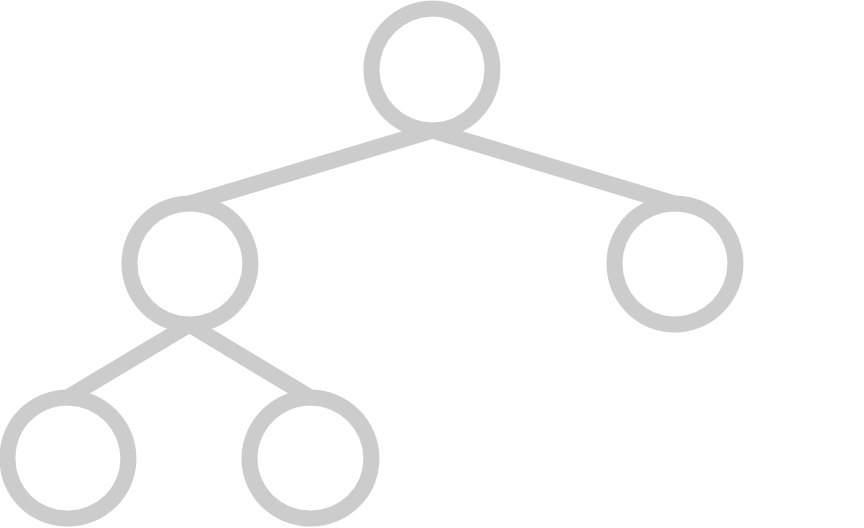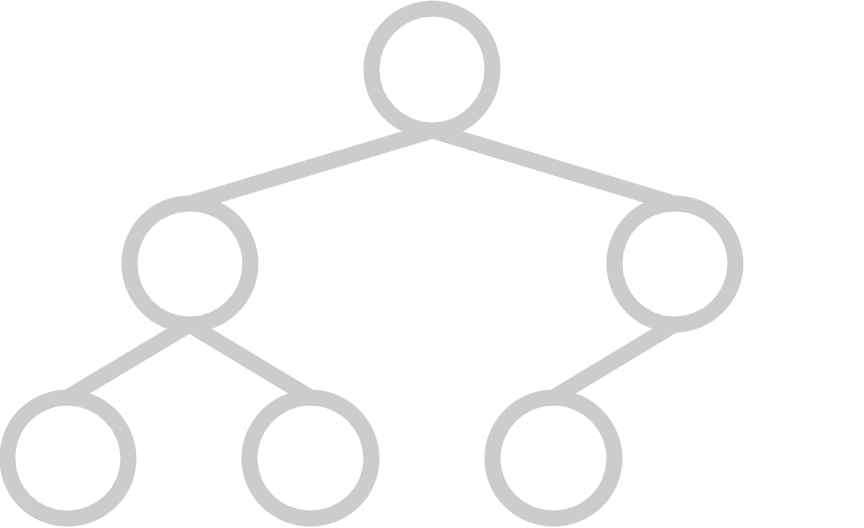And here are some examples of trees that are not complete:

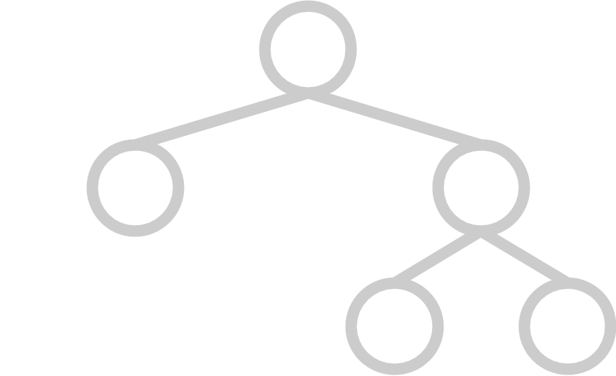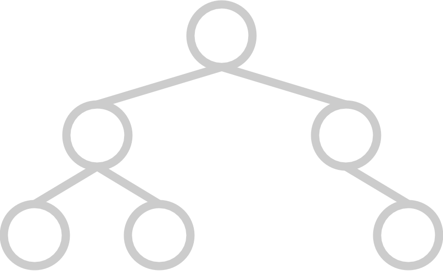Invariant 2: Heap Property #

Here is another property that will allow us to organize the heap in a way that will result in fast operations.

Every element must follow the heap property, which states that each element must be smaller than all of the elements in its subtree. This is known as the heap property.

If we have a heap, this guarantees that the element with the lowest value will always be at the root of the tree. If the elements are our priority values, then we are guaranteed that the element with the lowest priority value (the minimum) is at the root of the tree. This helps us access that item quickly, which is what we need for a (minimum) priority queue!

For the rest of this lab, we will be discussing the representation and operations of binary heaps. However, this logic can be modified to apply to heap heaps with any number of children.

Max Heap #

The heap we described is also known more specifically as a “min-heap”, because the heap property has the minimum element at the root at the root of the tree.

There is a variant of the heap data structure that is very similar: the max heap. Max heaps have the same completeness invariant, but have the opposite heap property. In a max heap, each element must be larger than all of the elements in its subtree. This means that the element with the highest priority value (the maximum) is at the root of the tree.

Java’s PriorityQueue uses a min-heap, but max-heap implementations exist.

Heap as `PriorityQueue` #

To use a heap as the underlying implementation of a priority queue, we can use the priority values of each of the priority queue’s items as the elements inside our heap. This way, the lowest or highest priority value object will be at the top of the heap, and the priority queue’s peek operation will be very fast.

Heap Representation #

In Project 1, we discovered that deques could be implemented using arrays or linked nodes. It turns out that this dual representation extends to trees as well! Trees are generally implemented using nodes with parent and child links, but they can also be represented using arrays.

Here’s how we can represent a binary tree using an array:

HeapArray

The root of the tree will be in position 1 of the array (nothing is at position 0).
The left child of a node at position \(N\) is at position \(2N\).
The right child of a node at position \(N\) is at position \(2N + 1\).
The parent of a node at position \(N\) is at position \(N / 2\).

Because binary heaps are essentially binary trees, we can use this array representation to represent our binary heaps!

Note: this representation can be generalized to trees with any variable number of children, not only binary trees.

You might have asked why we placed the root at 1 instead of 0. We do this for this is to to make indexing more convenient. If we had placed the root at 0, then our calculations would be:

The left child of a node at position \(N\) is at position \(2N + 1\).
The right child of a node at position \(N\) is at position \(2N + 2\).
The parent of a node at position \(N\) is at position \((N - 1) / 2\).

Unless otherwise specified we will place the root at position 1 to make the math slightly cleaner.

Heap Operations #

For min heaps, there are three operations that we care about:

findMin: Returning the lowest value without removal. (If we were using our min heap to implement a priority queue, this would correspond to accessing the highest priority element.)
insert: Inserting an element to the heap.
removeMin: Removing and returning the item with the lowest value. (If we were using our min heap to implement a priority queue, this would correspond to removing and returning the highest priority element.)

When we do these operations, we need to make sure to maintain the invariants mentioned earlier (completeness and the heap property). Let’s walk through how to do each one.

`findMin` #

The element with the smallest value will always be stored at the root due to the min-heap property. Thus, we can just return the root node, without changing the structure of the heap.

`insert` #

Put the item you’re adding in the next available spot in the bottom row of the tree. If the row is full, make a new row. This is equivalent to placing the element in the next free spot in the array representation of the heap. This ensures the completeness of the heap because we’re filling in the bottom-most row left to right.
If the element that has just been inserted is N, swap N with its parent as long as N is smaller than its parent or until N is the new root. If N is equal to its parent, you can either swap the items or not.

This process is called bubbling up (sometimes referred to as swimming), and this ensures the min-heap property is satisfied because once we finish bubbling N up, all elements below N must be greater than it, and all elements above must be less than it.

Here is iterative pseudocode for the bubble-up process:
```
bubbleUp(index) {
   while (index is not the root and arr[index] is smaller than parent) {
      swap arr[index] with arr[parent]
      update index to parent
   }
}
```

`removeMin` #

Swap the element at the root with the element in the bottom rightmost position of the tree. Then, remove the bottom rightmost element of the tree (which should be the previous root and the minimum element of the heap). This ensures the completeness of the tree.
If the new root N is greater than either of its children, swap it with that child. If it is greater than both of its children, choose the smaller of the two children. Continue swapping N with its children in the same manner until N is smaller than its children or it has no children. If N is equal to both of its children or is equal to the lesser of the two children, you can choose to swap the items or not. Typically we would choose to not, as doing so would be unnecessary work and our algorithm might be marginally faster if we skip this work.

This is called bubbling down (sometimes referred to as sinking), and this ensures the min-heap property is satisfied because we stop bubbling down only when the element N is less than both of its children and also greater than its parent.

Here is iterative pseudocode for the bubble-down process:
```
bubbleDown(index) {
   while (there is a child and arr[index] is greater than either child) {
      swap arr[index] with the SMALLER child
      update index to the index of the swapped child
   }
}
```

Heaps Visualization #

If you want to see an online visualization of heaps, take a look at the USFCA interactive animation of a min heap. You can type in numbers to insert, or remove the min element (ignore the BuildHeap button for now; we’ll talk about that later this lab) and see how the heap structure changes.

Discussion: Heaps Practice and Runtimes #

Min Heap Operations #

Assume that Heap is a binary min-heap (smallest value on top) data structure that is a properly-implemented heap. Draw the heap and its corresponding array representation after all of the operations below have occurred. Characters are compared in alphabetical order.

Heap<Character> h = new Heap<>();
h.insert('f');
h.insert('h');
h.insert('d');
h.insert('b');
h.insert('c');
h.removeMin();
h.removeMin();

Answers (click to expand):

Heap as a tree:

   d
  / \
 h   f

Heap as an array: [-,'d','h','f']

(- denotes the absence of the first element)

Runtimes #

Now that we’ve gotten the hang of the methods, let’s evaluate the worst case runtimes for each of them! Consider an array-based min-heap with \(N\) elements. As we insert elements, the backing array will run out of space and need to be resized. If we ignore the cost of resizing the array, what is the worst case asymptotic runtime of each of the following operations?

findMin
insert
removeMin

Answers (click to expand):

findMin: \(\Theta(1)\)
insert: \(\Theta(\log N)\), because we may bubble up through \(\log N\) layers
removeMin: \(\Theta(\log N)\), because we may bubble down through \(\log N\) layers

Now consider those same operations but also include the effects of resizing the underlying array or ArrayList. You should answer this question for the operations insert, removeMin, and findMin. Also assume that we will only resize up and we will not resize down.

Answers (click to expand):

findMin: \(\Theta(1)\)
insert: \(Theta(N)\), because resizing takes linear time
removeMin: \(\Theta(\log N)\), because we don’t resize down

`PriorityQueue` Implementation #

Now, let’s implement what we’ve just learned about priority queues and heaps! There are a few files given to you in the skeleton, which will be broken down here for you:

PriorityQueue.java: This interface represents our priority queue, detailing what methods we want to exist in our PQ.
MinHeap.java: This class represents our array-backed binary min heap.
MinHeapPQ.java: This class represents a possible implementation of a priority queue, which will use our MinHeap to implement the PriorityQueue interface.

We will start with implementing our MinHeap and then move onto MinHeapPQ. You do not have to do anything with PriorityQueue (it has been provided for you).

Exercise: `MinHeap` #

Representation #

In the MinHeap class, implement the array-based representation of a heap discussed above by implementing the following methods:

private int getLeftOf(int index);
private int getRightOf(int index);
private int getParentOf(int index);
private int min(int index1, int index2);

Our code will use an ArrayList instead of an array so we will not have to resize our array manually, but the logic is the same. In addition, make sure to look through and use the methods provided in the skeleton (such as getElement) to help you implement the methods listed above!

Operations #

After you’ve finished the methods above, fill in the following missing methods in MinHeap.java. We recommend doing these methods in order.

public E findMin();
private void bubbleUp(int index);
private void bubbleDown(int index);
public void insert(E element);
public int size();
public E removeMin();

When you implement insert and removeMin, you should be using bubbleUp and/or bubbleDown, and when you implement bubbleUp and bubbleDown, you should be using the methods you wrote above (such as getLeft, getRight, getParent, and min) and the ones provided in the skeleton (such as swap and setElement).

It is highly recommended to use the swap and setElement methods if you ever need to swap the location of two items or add a new item to your heap. This will help keep your code more organized and make the next task of the lab a bit more straightforward. Additionally, this reinforces the abstraction barrier, which we love in CS61BL! When possible, don’t break the abstraction barrier.

Remember that we have provided pseudocode for bubbleUp and bubbleDown above.

Usually MinHeap’s should be able to contain duplicates but for the insert method, assume that our MinHeap cannot contain duplicate items. To do this, use the contains method to check if element is in the MinHeap before you insert. If element is already in the MinHeap, throw an IllegalArgumentException. We’ll talk about how to implement contains in the next section.

Before moving on to the next section, we suggest that you test your code! We have provided a blank MinHeapTest.java file for you to put any JUnit tests you’d like to ensure the correctness of your methods.

Exercise: `update` and `contains` #

We have two more methods that we would like to implement (contains and update) whose behaviors are described below:

update(E element): Sometimes, priorities change. Our heap invariant can be violated if an element’s priority changes while it is in the heap. If element is in the MinHeap, replace the MinHeap’s version of this element with element and update its position in the MinHeap.
contains(E element): Checks if element is in our MinHeap.

Let’s take a look at the update method first.

`update(E element)` #

The update(E element) method will consist of the following four steps:

Check if element is in our MinHeap.
If so, find the element in our MinHeap (by finding the index the element is at).
Replace the element with the new element.
Bubble element up or down depending on how it was changed since its initial insertion into the MinHeap.

Unfortunately, Steps 1 and 2 (checking if our element is present and finding the element) are actually nontrivial linear time operations since heaps are not optimized for this operation. To check if our heap contains an item, we’ll have to iterate through our entire heap, looking for the item (see “Search”’s runtime here). There is a small optimization that we can make for this part if we know we have a max heap, but this would in general make our update method run in at least linear time.

This is not extremely bad, but applications of our heap would really benefit from having a fast update method.

We can get around this by introducing another data structure to our heap! Though this would increase the space complexity of the heap and is not how Java implements PriorityQueue, it will be worth the runtime speedup of our update method in any applications of our heap.

We would essentially want to use this extra data structure to speed to help us make step 1 (checking if our MinHeap contains a particular element) and step 2 (get the index corresponding to a particular element) fast.

In order to implement this new optimized version you may need to update some methods in order to ensure that this data structure always has accurate information. There is no need to implement these optimization for this lab, but they would be needed in any large scale use of your data structure.

Implement update(E element) according to the steps listed above. Remember if element is not in the MinHeap, you should throw a NoSuchElementException. The optimized update(E element) operation is not required for credit on this lab.

`contains(E element)` #

Now, implement contains(E element).

Note that if you do choose to implement the optimized approach we have hinted at above, you can use the same data structure to implement a faster contains operation!

Exercise: `MinHeapPQ` #

Now let’s use the MinHeap class to implement our own priority queue! We will be doing this in our MinHeapPQ class.

Take a look at the code provided for MinHeapPQ, a class that implements the PriorityQueue interface. In this class, we’ll introduce a new wrapper class called PriorityItem, which wraps the item and priorityValue in a single object. This way, we can use PriorityItem’s as the elements of our underlying MinHeap.

Before you start implementing these methods, we recommend that you write your tests! Long live TDD! Just like with MinHeap, we have provided a blank MinHeapPQTest.java file so you can write JUnit tests to ensure your code is working properly.

Then, implement the remaining methods of the interface (duplicated below) of the MinHeapPQ class:

public T peek();
public void insert(T item, double priority);
public T poll();
public void changePriority(T item, double priority);
public int size();

For the changePriority method, use the update method from the MinHeap class. The contains method has already been implemented for you.

Note: you shouldn’t have to write too much code in this file. Remember that your MinHeap will do most of the work for you! Our solution only requires 5 line changes from the provided skeleton. It is of course fine if you use more lines but you should not be writing long functions for this. Instead, rely on the corresponding MinHeap methods.

`compareTo()` vs `.equals()` #

You may have noticed that the PriorityItem has a compareTo method that compares priority values, while the equals method compares the items themselves. Because of this, it’s possible that compareTo will return 0 (which usually means the items that we are comparing are equal) while equals will still return false. However, according to the Javadocs for Comparable:

It is strongly recommended, but not strictly required that (x.compareTo(y) == 0) == (x.equals(y)). Generally speaking, any class that implements the Comparable interface and violates this condition should clearly indicate this fact. We will require this from you in CS61BL, but it is vital to know this requirement does not hold for real world programmers!

Thus, our PriorityItem class “has a natural ordering that is inconsistent with equals”. Normally, we would want x.compareTo(y) == 0 and x.equals(y) to both return true for the same two objects, but this class will be an exception. Make sure to clearly note this exception in the documentation of your code!

Discussion: Heap Brainteasers #

Now, let’s get into some deeper questions about heaps.

Heaps and BSTs #

Consider binary trees that are both max heaps and binary search trees.

How many nodes can such a tree have? Choose all that apply.

1 node
2 nodes
3 nodes
4 nodes
5 nodes
Any number of nodes
No trees exist

Answer (click to expand):

Such a tree can either have either 1 node or 2 nodes.

Determining Completeness #

It’s not obvious how to verify that a binary tree is complete (assuming it is represented using children links rather than an array as we have discussed in this lab). A CS 61BL student suggests the following recursive algorithm to determine if a tree is complete:

A one-node tree is complete.
A tree with two or more nodes is complete if its left subtree is complete and has depth \(k\) for some \(k\), and its right subtree is complete and has depth \(k\) or \(k - 1\).

Here are some example trees. Think about whether or not the student’s proposed algorithm works correctly on them.

sample-trees

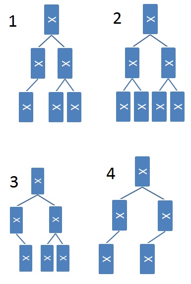
Choose all that apply to test your understanding of the proposed algorithm.

Tree 1 is complete
Tree 1 would be identified as complete
Tree 2 is complete
Tree 2 would be identified as complete
Tree 3 is complete
Tree 3 would be identified as complete
Tree 4 is complete
Tree 4 would be identified as complete

Answer (click to expand):

The correct answers are:

“Tree 1 would be identified as complete”
“Tree 2 is complete”
“Tree 2 would be identified as complete”
“Tree 4 would be identified as complete”.

Third Biggest Element in a Max Heap #

Here’s an example max heap.

third-largest

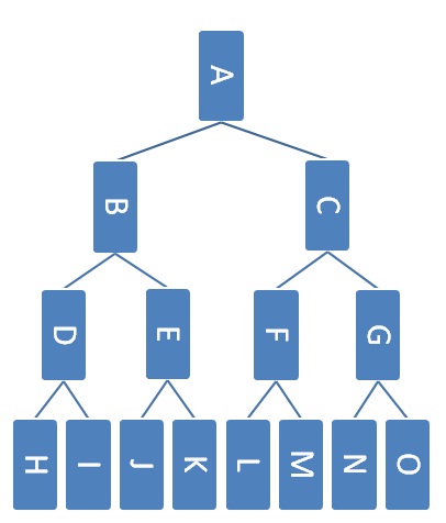
Which nodes could contain the third largest element in the heap assuming that the heap does not contain any duplicates?

Answer (click to expand):

Nodes: B, C, D, E, F, and G.

Which nodes could contain the third largest element in the heap assuming that the heap can contain duplicates?

Answer (click to expand):

Nodes: A, B, C, D, E, F, G, H, I, J, K, L, M, N, and O.

Conclusion #

In today’s lab, we learned about another abstract data type called the priority queue. Priority queues can be implemented in many ways, but are often implemented with a binary min heap. It is very easy to conflate the priority queue abstract data type and the heap data structure, so make sure to understand the difference between the two!

Additionally, we learned how to represent a heap with an array, as well as some of its core operations. We then explored a few conceptual questions about heaps.

All in all, priority queues are an integral component of many algorithms for graph processing (which we’ll cover in a few labs). For example, in the first few weeks of CS 170, Efficient Algorithms and Intractable Problems, you will see graph algorithms that use priority queues. Look out for priority queues in other CS classes as well! You’ll find them invaluable in the operating systems class CS 162, where they’re used to schedule which processes in a computer to run at what times.

Deliverables #

To receive credit for this lab:

Complete MinHeap.java
Complete MinHeapPQ.java

FAQ #

Before You Begin #

Priority #

Priority vs. Priority Values #

Priority Queues #

Discussion: PQ Implementations #

Heaps #

Heap Properties #

Invariant 1: Completeness #

Invariant 2: Heap Property #

Max Heap #

Heap as PriorityQueue #

Heap Representation #

Heap Operations #

findMin #

insert #

removeMin #

Heaps Visualization #

Discussion: Heaps Practice and Runtimes #

Min Heap Operations #

Runtimes #

PriorityQueue Implementation #

Exercise: MinHeap #

Representation #

Operations #

Exercise: update and contains #

update(E element) #

contains(E element) #

Exercise: MinHeapPQ #

compareTo() vs .equals() #

Discussion: Heap Brainteasers #

Heaps and BSTs #

Determining Completeness #

Third Biggest Element in a Max Heap #

Conclusion #

Deliverables #

Heap as `PriorityQueue` #

`findMin` #

`insert` #

`removeMin` #

`PriorityQueue` Implementation #

Exercise: `MinHeap` #

Exercise: `update` and `contains` #

`update(E element)` #

`contains(E element)` #

Exercise: `MinHeapPQ` #

`compareTo()` vs `.equals()` #