Introduction

This project was originally created by former TA and CS 61BL instructor Alan Yao (now at AirBNB). It is a web mapping application inspired by Alan’s time on the Google Maps team and the OpenStreetMap project, from which the tile images and map feature data was downloaded.

In this project, you’ll build the “smart” pieces of a web-browser based Google Maps clone. In this project you will be implementing and extending a few data structures and algorithms we have already learned about in this class. Namely, you will implement a \(k\)-d tree from lab 15, extend your MinHeapPQ from lab 17, and implement the A* algorithm which will be introduced in lab 19.

Unlike prior 61BL projects, you’ll start with a gigantic code base that somebody else wrote. This is typical in real world programming, where you don’t have the luxury and freedom that comes with starting from totally blank files. As a result, you’ll need to spend some time getting to know the provided code, so that you can complete the parts that need completing.

By the end of this project, with some extra work, you can even host your application as a publicly available web app! More details will be provided at the end of this spec.

There is a reference version of the project solution running at http://bearmaps-su20-s1.herokuapp.com/map.html. It will probably be quite slow given that lots of people will be using it.

Setup

Libraries

Start by pulling from skeleton as you do before all labs and projects. Once you’ve gotten your proj3 directory, cd into the library-su20 directory and do the following commands (this will take a long time because there are 20,000+ files to download):

git submodule update --init

After doing this, check that the following are true:

• You should have the javalib folder from before and a new data folder in library-su20.
• There should be library-su20/data/proj3_imgs, library-su20/data/proj3_xml, and library-su20/data/proj3_test_inputs folders.
• There should be a library-su20/javalib/proj3 folder, in addition to the other libraries.

IntelliJ Setup

Importing the Project and Libraries

Start by importing the project as usual (using either File->New->Project From Existing Sources or “Import or Open” on the front panel).

Next, we’ll need to import all the libraries that are in the javalib folder, including the proj3 directory. If you do not remember how to do this, do the following steps.

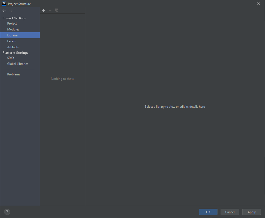
To do this, click “File->Project Structure”, then click “Libraries” on the screen that pops up. You should see something like what is shown in the figure below.

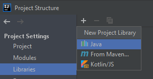
The next step is to click the plus sign at the top of the screen, then click “Java” from the list of options.

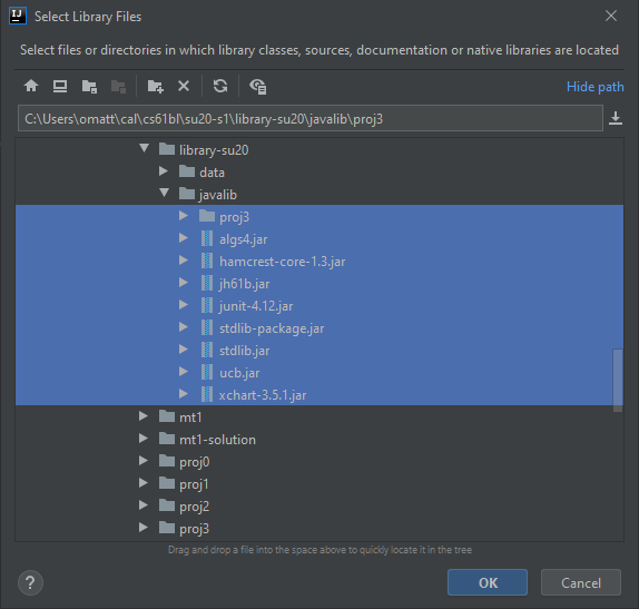
Navigate to the library-su20 folder and click all the files in that folder.

Click “OK” and a message should pop up saying “Library ‘proj3’ will be added to the selected modules: proj3”.

Click “OK” again. Then click “OK” one more time.

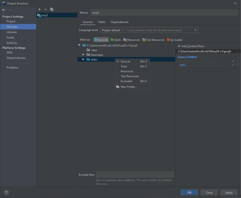
Marking the Static Directory

Go to Project Structure -> Modules -> proj3. Right-click the static folder and select Sources

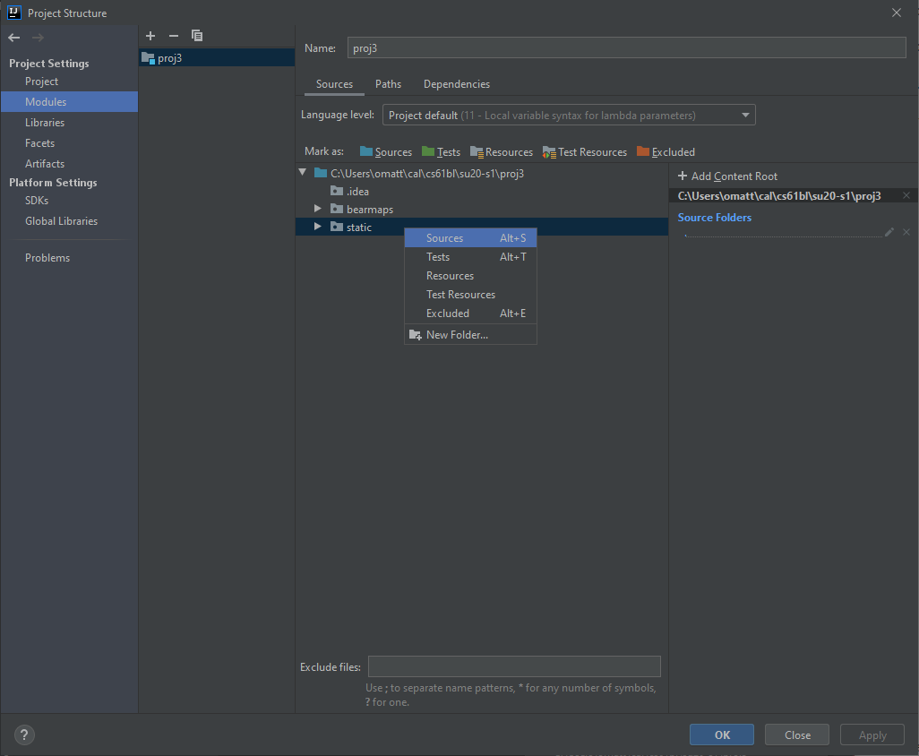
The static folder should now be highlighted in blue.

Setting the Language Level

Depending on your version of IntelliJ you may need need to do this step, but it doesn’t hurt to do so anyway.

Again, do “File->Project Structure”. Then click “Project”, which is just a bit above the “Libraries” button. Then under “Project Language Level”, make sure that level 11 is selected.

Verifying Project 3 Setup

To finally verify that everything is working correctly, open the java file called bearmaps/MapServer.java and run its main method.

It should start running, and in the console, you should see something similar to the following:

[Thread-0] INFO org.eclipse.jetty.util.log - Logging initialized @1829ms to org.eclipse.jetty.util.log.Slf4jLog
[Thread-0] WARN org.eclipse.jetty.server.AbstractConnector - Ignoring deprecated socket close linger time
[Thread-0] INFO spark.webserver.JettySparkServer - == Spark has ignited ...
[Thread-0] INFO spark.webserver.JettySparkServer - >> Listening on 0.0.0.0:4567
[Thread-0] INFO org.eclipse.jetty.server.Server - jetty-9.4.15.v20190215; built: 2019-02-15T16:53:49.381Z; git: eb70b240169fcf1abbd86af36482d1c49826fa0b; jvm 11.0.6+10
[Thread-0] INFO org.eclipse.jetty.server.session - DefaultSessionIdManager workerName=node0
[Thread-0] INFO org.eclipse.jetty.server.session - No SessionScavenger set, using defaults
[Thread-0] INFO org.eclipse.jetty.server.session - node0 Scavenging every 600000ms
[Thread-0] INFO org.eclipse.jetty.server.AbstractConnector - Started ServerConnector@b931a75{HTTP/1.1,[http/1.1]}{0.0.0.0:4567}
[Thread-0] INFO org.eclipse.jetty.server.Server - Started @2212ms

If you’re using Windows, a pop-up might appear saying “Windows Defender Firewall has blocked some features of this app.”. If this happens, you should allow access.

What’s happening here is that your computer is now acting as a web server, with your Java code ready to respond to web requests. Let’s see it in action.

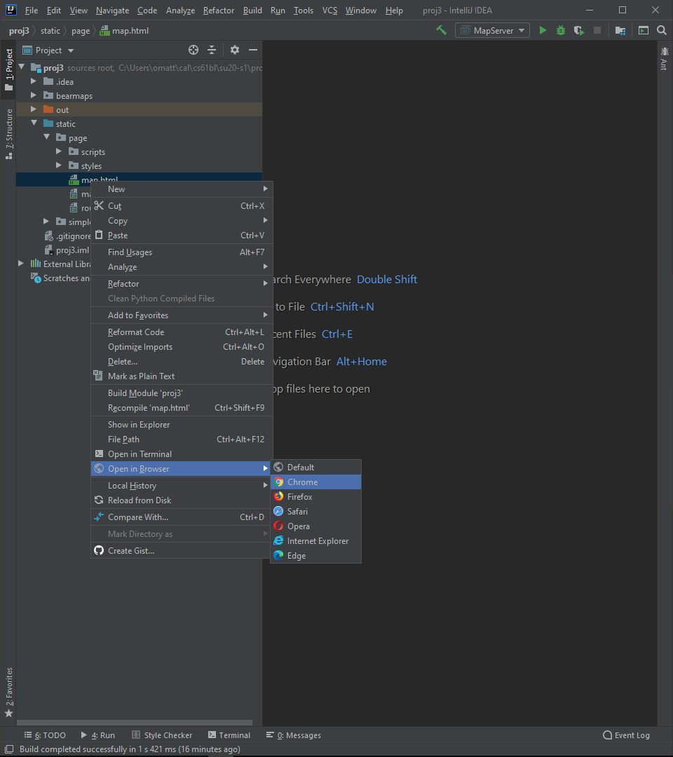
Go to the file navigation panel on the left side of IntelliJ and look for static/page towards the bottom of your project directory. Expand it, and you should see map.html. Right click on this file, then go to “Open in Browser”, similar to shown below. We recommend Chrome.

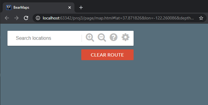
Once you’ve opened map.html, you should see something like the window below, where the front end makes a back end to provide image data. Since you haven’t implemented the back end, this data will never arrive.

You’ll also notice that in the console, opening up map.html in the web browser did something. Specifically you should see the message below.

Since you haven't implemented RasterAPIHandler.processRequest, nothing is displayed in your browser.
Your rastering result is missing the render_grid field.

Let’s try one more thing! Go to the processRequest method of the RasterAPIHandler method of the bearmaps.server.handler.impl package and you’ll see the following print statements. Try uncommenting the two print statements in the file (replicated below):

System.out.println("yo, wanna know the parameters given by the web browser? They are:");
System.out.println(requestParams);

Stop (using the red stop button in IntelliJ, or using the method of your choice) the MapServer program and restart it. Then refresh the page in your web browser and you should see this printed in IntelliJ:

yo, wanna know the parameters given by the web browser? They are:
{lrlon=-122.19016181945801, ullon=-122.27625, w=2006.0, h=1008.0, ullat=37.88, lrlat=37.84584557684252}
Since you haven't implemented RasterAPIHandler.processRequest, nothing is displayed in your browser.
Your rastering result is missing the render_grid field.

Pretty cool! Your web browser is trying to communicate with your Java program! In this project, you’ll be modifying your Java code so that it is able to talk to the browser and display mapping data.

Phew! That’s all the setup we need. Now we can get started on the project itself.

Note: Absolutely make sure to end your instance of MapServer before re-running or starting another up.** Not doing so will cause a java.net.BindException: Address already in use. If you end up getting into a situation where you computer insists the address is already in use, either figure out how to kill all Java processes running on your machine (using Stack Overflow or similar) or reboot your computer.

Overview

The project 2C video playlist from the Spring 2019 offering of CS 61B starts with an introductory video that should help you get started. Though this project has been augmented since it was done last Spring, the video and slides are still quite relevant. The slides that will be used in the project 2C video playlist are available here.

Application Structure

Your job for this project is to implement the back end of a web server. To use your program, a user will open an html file in their web browser that displays a map of the city of Berkeley, and the interface will support scrolling, zooming, and route finding (similar to Google Maps). We’ve provided all of the “front end” code. Your code will be the “back end” which does all the hard work of figuring out what data to display in the web browser.

At its heart, the project works like this: The user’s web browser provides a URL to your Java program, and your Java program will take this URL and generate the appropriate output, which will displayed in the browser. For example, suppose your program were running at bloopblorpmaps.com, the URL might be:

bloopblorpmaps.com/raster&ullat=37.89&ullon=-122.29&lrlat=37.83&lrlon=-122.22&w=700&h=300

The job of the back end server (i.e. your code) is take this URL and generate an image corresponding to a map of the region specified inside the URL (more on how regions are specified later). This image will be passed back to the front end for display in the web browser.

You’ll notice the web address that we saw in the setup instructions is strange, starting with localhost:63365 or similar instead of something like www.eecs.berkeley.edu. localhost means that the website is on your own computer, and the 63365 refers to a port number, something that you’ll probably learn about in a future class.

We will be providing the front end (in the form of HTML and Javascript files which you will not need to open or modify), but we’ll also provide a great deal of starter code (in the form of .java files) for the back end. This starter code will handle all URL parsing and communication for the front end. This code uses Java Spark as the server framework. You don’t need to worry about the internals of this, since our code handles all the messy translation between web browser and your Java programs.

If you do go exploring, you’ll notice that the structure of the skeleton code for this project is significantly more complex than anything you’ve probably seen in a class. This is because we’ve built something that more closely resembles what you might see in a real world project, with tons of different packages interesting in various ways. You’re not required to understand all of this in order to complete the project, though you’re welcome to explore. The next section of this spec will explain what pieces you absolutely have to look at.

Parts of this Project

There are 6 parts of this project. The first three are required, the fourth is extra credit, and the last two are completely optional. The parts are as follows:

• Part I, Map Rastering: Given coordinates of a rectangular region of the world and the size of the web browser window, provide images of the appropriate resolution that cover that region.
• Part II, Data Structures: Implementing a \(k\)-d tree and extending the MinHeapPQ to be used in Part III.
• Part III, Routing: Given a start and destination latitude and longitude, provide street directions between those points.
• Part IV, Autocomplete: Given a string, find all locations that match that string. Useful for finding, e.g. all the Top Dogs in Berkeley.
• Part V, Written Directions: Augment the routing from Part III to include written driving directions.
• Part VI, Above and Beyond: Do anything else that seems fun.

I. Map Rastering (Required)

Rastering is the job of converting information into a pixel-by-pixel image. In the bearmaps.server.handler.impl.RasterAPIHandler class you will take a user’s desired viewing rectangle and generate an image for them.

The user’s desired input will be provided to you as a Map<String, Double> params, and the main goal of your rastering code will be to create a String[][] that represents the image files that should be displayed in response to this query.

As a specific example (given as testTwelveImages.html in the skeleton files), the user might specify that they want the following information:

{lrlon=-122.2104604264636, ullon=-122.30410170759153, w=1085.0, h=566.0, ullat=37.870213571328854, lrlat=37.8318576119893}

This means that the user wants the area of earth delineated by the rectangle between longitudes -122.2104604264636 and -122.30410170759153 and latitudes 37.870213571328854 and 37.8318576119893. They also would like this area displayed in a window roughly 1085 x 566 pixels in size (width x height). We call the user’s desired display location on earth the query box.

To display the requested information, you will need street map pictures, which are provided in library-su20. All of the images provided are 256 x 256 pixels. Each image is at various levels of zoom. For example, the file d0_x0_y0.png is the entire map, and covers the entire region. The files d1_x0_y0.png, d1_x0_y1.png, d1_x1_y0.png, and d1_x1_y1.png are also the entire map, but at double the resolution, i.e. d1_x0_y0 is the northwest corner of the map, d1_x1_y0 is the northeast corner, d1_x0_y1 is the southwest corner, and d1_x1_y1 is the southeast corner.

More generally, at the \(D\)-th level of zoom, there are \(4^D\) images, with names ranging from dD_x0_y0 to dD_xk_yk, where \(k\) is \(2^D - 1\). As \(x\) increases from \(0\) to \(k\), we move eastwards, and as \(y\) increases from \(0\) to \(k\), we move southwards. Keep both of these points this in mind, as this will be useful when you write your rastering code!

The job of your rasterer class is decide, given a user’s query, which files to serve up. For the example above, your code should return the following 2D array of strings:

[[d2_x0_y1.png, d2_x1_y1.png, d2_x2_y1.png, d2_x3_y1.png],
[d2_x0_y2.png, d2_x1_y2.png, d2_x2_y2.png, d2_x3_y2.png],
[d2_x0_y3.png, d2_x1_y3.png, d2_x2_y3.png, d2_x3_y3.png]]

This means that the browser should display d2_x0_y1.png in the top left, then d2_x1_y1.png to the right of d2_x0_y1.png, and so forth. Thus our “rastered” image is actually a combination of 12 images arranged in 3 rows of 4 images each. Our code will then take your 2D array of strings and display the appropriate image in the browser. If you’re curious how this works, see writeImagesToOutputStream in RasterAPIHandler.

Since each image is 256 x 256 pixels, the overall “rastered” image given above will be 1024 x 768 pixels.

However, there are many combinations of images that cover the query box. For example, we could instead use higher resolution images of the exact same areas of Berkeley. For example, instead of using d2_x0_y1.png, we could have used d3_x0_y2.png, d3_x1_y2.png, d3_x0_y3.png, d3_x1_y3.png while also substituting d2_x1_y1.png by d3_x2_y2.png, d3_x3_y2.png, etc. The result would be total of 48 images arranged in 6 rows of 8 images each (make sure this makes sense!) and would result in a 2048 x 1536 pixel image.

It might be tempting to say that a 2048 x 1536 image is more appropriate than 1024 x 768. After all, the user requested 1085 x 556 pixels and 1024 x 768 is too small to cover the request in the width direction. However, pixel counts are not the way that we decide which images to use.

Instead, to rigorously determine which images to use, we will define the longitudinal distance per pixel (LonDPP) as follows. Given a query box or image, the LonDPP of that box or image is

\[\text{LonDPP} = \frac{\text{lower right longitude} - \text{upper left longitude}}{\text{width of the image (or box) in pixels}}\]

For example, for the query box in the example in this section, the LonDPP is (-122.2104604264636 + 122.30410170759153) / (1085) or 0.00008630532 units of longitude per pixel. At Berkeley’s latitude, this is very roughly 25 feet of distance per pixel.

Note that the longitudinal (horizontal) distance per pixel is not the same as the latitudinal (vertical) distance per pixel. This is because the earth is curved. If you use latDPP, you will have incorrect results.

The images that you return in your String[][] when rastering must be those that:

• Represent any region of the query box.
• Have the greatest LonDPP that is less than or equal to the LonDPP of the query box (as zoomed out as possible). If the requested LonDPP is less than what is available in the data files, you should use the lowest LonDPP available instead (i.e. depth 7 images).

For image depth 1 (e.g. d1_x0_y0), every tile has LonDPP equal to 0.000171661376953125 (for an explanation of why, see the next section) which is greater than the LonDPP of the query box, and is thus unusable. This makes intuitive sense as well: if the user wants an image which covers roughly 25 feet per pixel, we shouldn’t use an image that covers ~50 feet per pixel because the resolution is too poor. For image depth 2 (e.g. d2_x0_y1), the LonDPP is 0.0000858306884765625, which is better (i.e. smaller) than the user requested, so this is fine to use. For depth 3 tiles (e.g. d3_x0_y2.png), the LonDPP is 0.00004291534423828125. This is also smaller than the desired LonDPP, but using it is overkill since depth 2 tiles (e.g. d2_x0_y1) are already good enough. Think of LonDPP as “blurriness”, i.e. the d0 image is the blurriest (most zoomed out/highest LonDPP), and the d7 images are the sharpest (most zoomed in, lowest LonDPP).

As an example of an intersection query, consider the image below, which summarizes key parameter names and concepts. In this example search, the query box intersects 9 of the 16 tiles at depth 2.

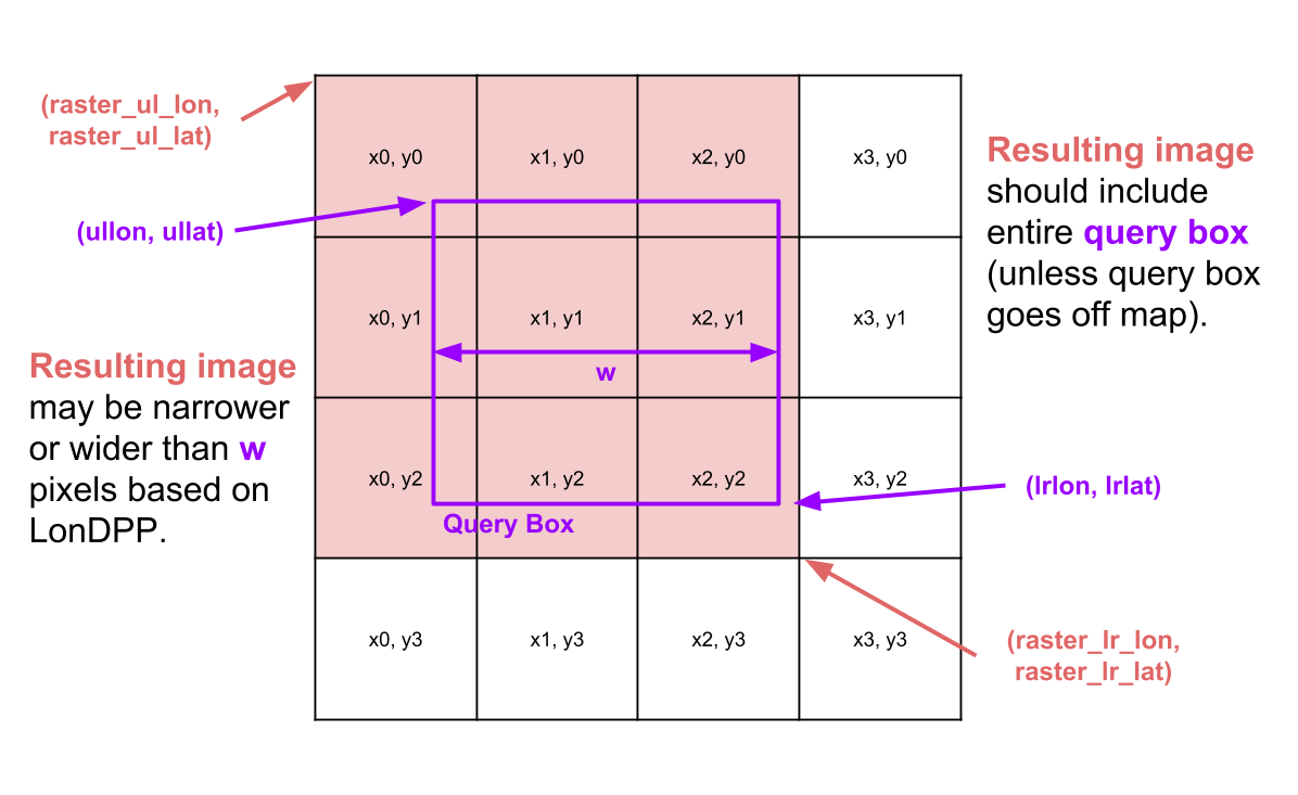
For an interactive demo of how the provided images are arranged, see this FileDisplayDemo. Try typing in a filename (.png extension is optional), and it will show what region of the map this file corresponds to, as well as the exact coordinates of its corners, in addition to the LonDPP in both longitude units per pixel and feet per pixel.

We do not take into account the curvature of the earth for rastering. The effect is too small to matter at the scale we are using (e.g. just the area surrounding the Berkeley campus). That is, we assume the LonDPP is the same for all values of y. In an industrial strength mapping application, we would need to keep in mind that the LonDPP per tile varies as we move with respect to the equator.

One natural question is, why not use the best quality images available all the time (i.e. smallest LonDPP, e.g. depth 7 images like d7_x0_y0.png)? The answer is that the front end doesn’t do any rescaling, so if we used ultra low LonDPPs for all queries, we’d end up with absolutely gigantic images displayed in our web browser. If we host this application on the web, that means sending massive files which puts more load on the server and might result in an overall slower application.

Image File Layout and “Bounding Boxes”

There are four constants that define the coordinates of the world map, all given in the bearmaps.utils.Constants.java class. The first is ROOT_ULLAT, which tells us the latitude of the upper left corner of the map. The second is ROOT_ULLON, which tells us the longitude of the upper left corner of the map. Similarly, ROOT_LRLAT and ROOT_LRLON give the latitude and longitude of the lower right corner of the map. All of the coordinates covered by a given tile are called the “bounding box” of that tile. So for example, the single depth 0 image d0_x0_y0 covers the coordinates given by ROOT_ULLAT, ROOT_ULLON, ROOT_LRLAT, and ROOT_LRLON.

Recommended exercise: Try opening d0_x0_y0.png. Then try using Google Maps to show the point given by ROOT_ULLAT, ROOT_ULLON. You should see that this point is the same as the top left corner of d0_x0_y0.png.

Another important constant in bearmaps.utils.Constants.java is TILE_SIZE. This is important because we need this to compute the LonDPP of an image file. For the depth 0 tile, the LonDPP is just (ROOT_LRLON - ROOT_ULLON)/TILE_SIZE, i.e. the number of units of longitude divided by the number of pixels.

All levels in the image library cover the exact same area. So for example, d1_x0_y0.png, d1_x1_y0.png, d1_x0_y1.png, and d1_x1_y1.png comprise the northwest, northeast, southwest, and southeast corners of the entire world map with coordinates given by the ROOT_ULLAT, ROOT_ULLON, ROOT_LRLAT, and ROOT_LRLON parameters.

The bounding box given by an image can be mathematically computed using the information above. For example, suppose we want to know the region of the world that d1_x1_y1.png covers. We take advantage of the fact that we know that d0_x0_y0.png covers the region between longitudes -122.29980468 and -122.21191406 and between latitudes 37.82280243 and 37.89219554. Since d1_x1_y1.png is just the southeastern quarter of this region, we know that it covers half the longitudinal and half the latitudinal distance as d0_x0_y0.png, specifically the region between longitudes -122.25585937 and -122.21191406 and between latitudes 37.82280243 and 37.85749898.

Similarly, we can compute the LonDPP in a similar way. Since d1_x1_y1.png is 256 x 256 pixels (as are all image tiles), the LonDPP is the difference of the longitudes of d1_x1_y1.png divided by TILE_SIZE ((-122.21191406 - -122.25585937)/256 or 0.00017166).

If you’ve fully digested the information described in the spec so far, you now know enough to figure out which files to provide given a particular query box. See the project 2C slides and video above for more hints if you’re stuck.

If someone is helping you who took 61B in Spring 2017 or earlier (this is getting less and less likely each semester), they might suggest using a Quadtree, which was the previously recommended way of solving the tile identification problem. You’re welcome to attempt this approach, but the project has changed enough that Quadtrees are no longer necessary nor desirable as a solution. It turns out that doing the math should in theory be faster than using this data structure–an important reminder that data structures are not always the answer.

Map Rastering (API)

In Java, you will implement the RasterAPIHandler by filling in a single method:

public Map<String, Object> processRequest(Map<String, Double> requestParams, Response response)

The given requestParams are described in the skeleton code. An example is provided in the “Map Rastering (Overview)” section above, and you can always try opening up one of our provided html files and simply printing out requestParams when this method is called to see what you’re given.

Your code should return a Map<String, Object> as described in the Javadocs (the /** */ comments in the skeleton code). We do this as a way to hack around the fact that Java methods can only return one value. This map includes not just the two dimensional array of Strings, but also a variety of other useful information that will be used by your web browser to display the image nicely (e.g. raster_lr_lon and raster_ul_lat). See the comments in the source code for more details. We will not explain these in the spec.

Corner Cases

Corner Case 1: Partial Coverage

For some queries, it may not be possible to find images to cover the entire query box. This is OK. This can happen in two ways:

• If the user goes to the edge of the map beyond where data is available.
• If the query box is so zoomed out that it includes the entire dataset.

In these cases, you should return what data you do have available.

Corner Case 2: No Coverage

You can also imagine that the user might provide query box for a location that is completely outside of the root longitude/latitudes. In this case, there is nothing to raster, raster_ul_lon, raster_ul_lat, etc. are arbitrary, and you should set query_success: false. If the server receives a query box that doesn’t make any sense, eg. ullon, ullat is located to the right of lrlon, lrlat, you should also ensure query_success is set to false.

Runtime

You may not iterate through / explore all tiles to search for intersections with the query box. Suppose there are \(k\) tiles intersecting a query box, and \(N\) tiles total. Your entire query should run in \(O(k)\) time. Your algorithm should not run in \(\Theta(N)\) time. This is not for performance reasons, since \(N\) is going to be pretty small in the real world (less than tens of thousands), but rather because the \(\Theta(N)\) algorithm is inelegant.

Warning

It is likely that you will get latitude and longitude or \(x\) and \(y\) mixed up at least once or mix up which way is up versus down for y. Remember that longitude corresponds to \(x\) and latitude corresponds to \(y\). Moving from west to east (left to right) increases \(x\) and moving from south to north (bottom to top) increases \(y\).

Testing

Java Tests

The bearmaps/test/java file contains four test files. For the purposes of testing Part I, you should try out TestRasterAPIHandler. We also provide TestRouter and TestRouterTiny for Part III, and TestDirections for part V.

These tests are to help save you time. In an ideal world, we’d have more time to get you to write these tests yourself so that you’d deeply understand them, but we’re giving them to you for free. You should avoid leaning too heavily on these tests unless you really understand them! The staff will not be able to explain individual test failures that are covered elsewhere in the spec, and you are expected to be able to resolve test failures using the skills you’ve been learning all semester to effectively debug.

Ineffective/inappropriate strategies for debugging: running the JUnit tests over and over again while making small changes each time, staring at the error messages and then posting on Ed asking what they mean rather than carefully reading the message and working to understand it.

Effective strategies include: using the debugger; reproducing the buggy inputs in a simpler file that you write yourself; rubber ducky debugging, etc.

You can feel free to modify these files however you want. We will not be testing your code on the same data as is given to you for your local testing - thus, if you pass all the tests in this file, you are not guaranteed to pass all the tests on the actual autograder.

Map Tests

It can be hard to use the provided map.html file to debug, since it involves user input and is generally complicated.

Thus, we’ve also provided html test files in the static/simple folder. These are test.html, testTwelveImages.html, and test1234.html that you can use to test your project without using the front-end. Whereas map.html is a fully featured interactive website, these special test html files make a hard-coded call to your RasterAPIHandler. You can modify the query parameters in these files. These files allow you to make a specific call easily.

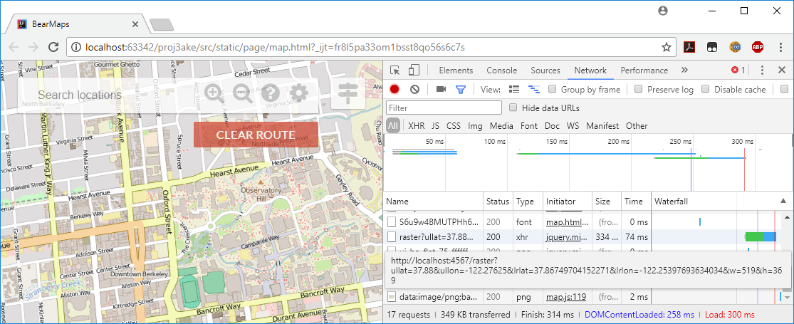
If you decide you want to debug using the fully featured map.html, you may find your browser’s Javascript console handy. For Chrome, if you right click then select “Inspect”, you will open the Chrome developer tools. Then click on the “Network” tab. All calls to your MapServer should be listed under type xhr and if you mouse-ver one of these xhr files you should be able to see the full query appear as follows:

You can also see the replies from your MapServer in the console tab, e.g. (click for higher resolution)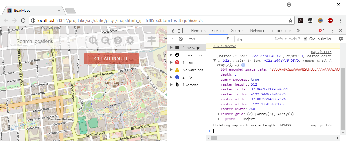

II. Data Structures (Required)

Before you proceed onto section three where we will implement Routing, we must first implement two data structures–a \(k\)-d tree and a MinHeapPQ. You should be familiar with both of these data structures from previous labs and lectures.

II(a). \(k\)-d Tree

For this part of the project, your primary goal will be to implement the KDTree class. This class implements a k-d tree as described in lecture 5 and in lab 15.

If you’re not familiar with how k-d trees work, please see Lecture 5 and lab 15 before proceeding. It is absolutely imperative that you do this before starting this assignment.

This will ultimately be useful in your Bearmaps application. Specifically, a user will click on a point on the map, and your \(k\)-d tree will be used to find the nearest intersection to that click.

If you need some help getting started, we will again refer you to the playlist of videos created by Josh Hug in spring 2019. The structure of the projects will be slightly different (e.g. in spring 2019 this was Project 2B), but the content should still remain relevant.

The walkthrough videos also includes links to a series of solutions videos, where in each video, Josh solves one part of the project. These videos cover some, but not all of this section of the project. Even if you solve this section entirely on your own, you still might find these solutions videos useful, so that you can compare your problem solving strategy to Josh.

Slides for this pseudo-walkthrough (including links to solution videos) can be found at this link. You are not required to follow these steps or use this walkthrough!

Provided Files

All of the work for this section of the project should be in the bearmaps.utils.ps package. Throughout this section we will not always include the full package name. We provide a class called Point.java that represents a location with an x and y coordinate. You should not modify this class. The methods in this class are:

• public double getX()
• public double getY()
• public static double distance(Point p1, Point p2)
• public boolean equals(Object o)
• public int hashCode()
• public String toString()

We also provide a interface called PointSet that represents a set of such points. It has only one method.

• public Point nearest(double x, double y): Returns the point in the set nearest to x, y.

NaivePointSet

Before you create your efficient KDTree class, you should first create a naive linear-time solution to solve the problem of finding the closest point to a given coordinate. The goal of creating this class is that you will have a alternative, albeit slower, solution that you can use to easily verify if the result of your \(k\)-d tree’s nearest is correct. Create a class called NaivePointSet. The declaration on your class should be:

    public class NaivePointSet implements PointSet {
        ...
    }

Your NaivePointSet should have the following constructor and method:

• public NaivePointSet(List<Point> points): You can assume points has at least size 1.
• public Point nearest(double x, double y): Returns the closest point to the inputted coordinates. This should take \(\theta(N)\) time where \(N\) is the number of points.

Note that your NaivePointSet class should be immutable, meaning that you cannot add or or remove points from it. You do not need to do anything special to guarantee this.

Our staff solution for this class is only 32 lines, and you should not be spending more than 1 to 2 hours to do this.

Example Usage

Point p1 = new Point(1.1, 2.2); // constructs a Point with x = 1.1, y = 2.2
Point p2 = new Point(3.3, 4.4);
Point p3 = new Point(-2.9, 4.2);

NaivePointSet nn = new NaivePointSet(List.of(p1, p2, p3));
Point ret = nn.nearest(3.0, 4.0); // returns p2
ret.getX(); // evaluates to 3.3
ret.getY(); // evaluates to 4.4

Part 2: K-d Tree

Now, create the class KDTree in a file KDTree.java. Your KDTree should have the following constructor and method:

• public KDTree(List<Point> points): You can assume points has at least size 1.
• public Point nearest(double x, double y): Returns the closest point to the inputted coordinates. This should take \(O(\log N)\) time on average, where \(N\) is the number of points.

As with NaivePointSet, your KDTree class should be immutable. Also note that while \(k\)-d trees can theoretically work for any number of dimensions, your implementation only has to work for the 2-dimensional case, i.e. when our points have only x and y coordinates.

For nearest, we recommend that you write a simple version and verify that it works before adding in the various optimizations from the pseudocode. For example, you might start by writing a nearest method that simply traverses your entire tree. Then, you might add code so that it always visits the “good” child before the “bad” child. Then after verifying that this works, you might try writing code that prunes the bad side. By doing things this way, you’re testing smaller ideas at once.

Defining Comparators Using Lambda Functions (Optional)

You may need to use comparators in this project for comparing objects. You can construct a concrete class that implements Comparator, or if you’d like, you can define a lambda function in Java. Remember the syntax for declaring a lambda for a comparator is:

Comparator<Type> function = (Type arg1, Type arg2) -> (...);
Comparator<Type> functionEquivalent = (arg1, arg2) -> (...);

where (...) is your desired return value that can use arguments arg1 and arg2.

Examples:

Comparator<Integer> intComparator = (i, j) -> i - j;
Comparator<Integer> intComparatorEquivalent = (i, j) -> {
  int diff = i - j;
  return diff;
};

You are not required to use a lambda but it will probably make your life slightly easier depending on how you approach the project.

Another handy tip: If you want to compare two doubles, you can use the Double.compare(double d1, double d2) method.

Testing NaivePointSet and KDTree

There are a number of different ways that you can construct tests for this part of the project, but we will go over our recommended approach.

Randomized Testing

Creating test cases that span all of the different edge cases will be difficult due to the complexity of the problem we are solving. To avoid thinking about all possible strange edge cases, we can turn towards techniques other than creating specific, deterministic tests to cover all of the possible errors. This might be similar to the fuzz tests you wrote in Project 1 (if you did write any).

Our suggestion is to use randomized testing which will allow you to test your code on a large sample of points which should encompass most, if not all, of the edge cases you might run into. By using randomized tests you can generate a large number of random points to be in your tree, as well as a large number of points to be query points to the nearest function. To verify the correctness of the results you should be able to compare the results of your KDTree’s nearest function to the results to the NaivePointSet’s nearest function. If we test a large number of queries without error we can build confidence in the correctness of our data structure and algorithm.

An issue is that randomized tests are not deterministic. This mean if we run the tests again and again, different points will be generated each time which will make debugging nearly impossible because we do not have any ability to replicate the failure cases. However, randomness in computers is almost never true randomness and is instead generated by pseudorandom number generators (PRNGs). Tests can be made deterministic by seeding the PRNG, where we are essentially initializing the PRNG to start in a specific state such that the random numbers generated will be the same each time. We suggest you use the class Random which will allow you to generate random coordinate values as well as provide the seed for the PRNG. More can be found about the specifications of this class in the online documentation.

Please put any tests you write in the provided KDTreeTest.java. You cannot share your tests with students other than your partner(s), but you are free to discuss testing strategies with them.

External Resources

Wikipedia is a pretty good resource that goes through nearest neighbor search in depth. You are free to reference pseudocode from course slides and other websites (use the @source tag to annotate your sources), but all code you write must be your own. We strongly recommend that you use the approach described in 61B, as it is simpler than described elsewhere.

You are welcome to look at source code for existing implementations of a k-d tree, though of course you should not be looking at solutions to this specific 61B project. Make sure to cite any sources you use with the @source tag somewhere in your code. As always you should not use other student’s solutions to this project as a source, e.g. a friend’s code, something you found on pastebin, etc.

Required Files for Part II(a)

You are required to submit the following files:

• NaivePointSet.java: your complete naive solution as described above.
• KDTree.java : your complete correct \(k\)-d tree implementation as described above.
• KDTreeTest.java: any tests you write for your \(k\)-d tree implementation. If you do not write any tests, you should still submit this file.

You are also welcome to submit other files.

Grading

NaivePointSet

We will only test your NaivePointSet for correctness, not efficiency.

\(k\)-d Tree

We will test your KDTree for correctness and efficiency. Correctness tests will be very similar to the randomized testing described in the Testing section, where we will compare your KDTree’s nearest results against our staff solution’s results. We will not be grading these based on efficiency, but please ensure that the method call completes in a reasonable about of time.

Efficiency tests will be similar to the correctness tests and will still require correctness, but they will also see how your solution performs with a very large number of points (hundreds of thousands) and many queries to nearest (tens of thousands). Your KDTree’s runtime will be compared to our staff KDTree’s runtime, and we will assign points based on that. If you implement the k-d tree correctly (similar to how you learn in lecture) and do not have repeated, redundant, or unnecessary function calls, you should be fine for these tests. For reference, our KDTree’s runtime while making 10,000 queries with 100,000 points is about 65-85x faster than our NaivePointSet’s runtime for the same points and queries. In addition, we will have a test that ensures your constructor is at most 10x slower than our staff KDTree’s constructor. This should not be a strict test as our constructor is relatively naive and doesn’t do anything fancier than what you learned in class.

II(b). MinHeapPQ

In lab 17, you should have created a MinHeapPQ class which implemented the PriorityQueue interface. For this part of the project we will be extending the existing class in order to implement several methods to have faster runtimes. This will be necessary to implement the AStarSolver in part III such that the runtime constraints will be met.

For much of this section you should be able to rely on your implementation from lab 17 as a starting point. This by no means is a requirement and you may start again if you would like. The instructions provided below describe the creation of the MinHeapPQ again and are somewhat redundant to the lab.

The primary difference between this part of the project and the lab is that here you will need to meet stricter runtime requirements. Be careful to make sure that you have followed the runtime constraints or you will likely run into issues with tests for this section and for later parts of the project.

PriorityQueue Interface

Your MinHeapPQ should implement the PriorityQueue. The operations are described below:

• public T peek(): Returns but does not remove the highest priority element. If no items exist, throw a NoSuchElementException.
• public void insert(T item, double priorityValue): Inserts item into the PriorityQueue with priority value priorityValue. If the item already exists, throw an IllegalArgumentException. You may assume that item is never null.
• public T poll(): Removes and returns the highest priority element. If no items exist, throw a NoSuchElementException.
• public void changePriority(T item, double priorityValue): Changes the priority value of item to priorityValue. Assume the items in the PriorityQueue are all distinct. If the item does not exist, throw a NoSuchElementException.
• public int size: Return the number of items in the PriorityQueue.
• public boolean contains(T item): Returns true if item is in the PriorityQueue.

There are a few key things to keep in mind regarding this interface:

• The priority is extrinsic to the object. That is, rather than relying on some sort of comparison function to decide which item is less than another, we simply assign a priority value using the insert or changePriority functions.
• There is an additional changePriority function that allows us to set the extrinsic priority of an item after it has been added.
• There is a contains method that returns true if the given item exists in the PQ (not all priority queues have this function).
• There may only be one copy of a given item in the priority queue at any time. To be more precise, if you try to add an item that is equal to another according to .equals(), the PQ should throw an exception.
• If there are 2 items with the same priority, you may break ties arbitrarily.

Provided Files

We have provided an additional NaiveMinPQ, which is a slow but correct implementation of this interface. contains, peek and poll use built in ArrayList or Collections methods to do a brute force search over the entire ArrayList. This takes time proportional to the length of the list, and each of these operations will have worst case \(\Theta(N)\) runtime.

The only small discrepancy there is between the NaiveMinPQ and the correct behavior is that this implementation does not throw the correct exception for the insert method. This is because this exception would make this class too slow to be usable for comparing runtimes with our implementation.

MinHeapPQ

Your job for this part of the project is to create (or update) the MinHeapPQ class, which must implement the PriorityQueue interface.

Your MinHeapPQ is subject to the following rules. Please note that some of these constraints are stricter that what we required in lab 17. You may need to edit either MinHeap or MinHeapPQ to resolve the differences.

• One of your instance variables should be a MinHeap. It is OK to have additional private variables in either MinHeap or MinHeapPQ.
• Your peek, contains, size and changePriority methods must run worst case \(\Theta(\log(N))\) time. Your insert and poll must run in \(\Theta(\log(N))\) average time, i.e. they should be logarithmic, except for the rare resize operation. For reference, when making 1000 queries on a heap of size 1,000,000, our solution is about 300x faster than the naive solution. Iterating over the ArrayList in MinHeap for any of these methods will be linear time and thus too slow!
• You may not add additional public methods. Private methods or “package private” methods are fine.

We have not discussed how you should implement the changePriority method in lab or lecture. You’ll have to invent this yourself. You may discuss your approach at a high level with other students (e.g. drawing out diagrams), but you should not share or look at each other’s code, nor should you work closely enough that your code may resemble each other’s.

Testing MinHeapPQ

You again will be responsible for writing your own tests and ensuring the correctness of your code! You may not share tests with any other students - please ensure that all code in your possession, including tests, were written by you. You should write any additional tests in the provided file MinHeapPQTest.java.

If you’re not sure how to start writing tests, some tips follow. Feel free to follow them or ignore them

1. We encourage you to primarily write tests that evaluate correctness based on the outputs of methods that provide output (e.g. peek and poll). This is in contrast to tests that try to directly test the states of instance variables (see tip #3 below). For example, to test changePriority, you might use a sequence of insert operations, a changePriority call, and then finally check the output of a poll call. This is (usually) a better idea than iterating over your private variables to see if changePriority is setting some specific instance variable. Don’t violate abstraction barriers!

2. Write tests for functions in the order that you write them. You might even find it helpful to write the tests first, which can help elucidate the task you’re trying to solve. Since each function may call previously written functions, this helps ensure that you are building a solid foundation.

3. If you want to write tests that require looking inside of your private instance variables, these tests should be part of the MinHeapPQ or MinHeap class itself. For example, if you want to write a test that only calls the insert method, there’s no way to write a test in the manner suggested in tip #1. It’s debatable whether or not you should even write such tests, since tests of type #1 should ideally catch any errors. Follow your heart.

4. If you have helper methods you’d like to test, you can either include the tests in MinHeapPQ, or you should make those helper methods “package private”. To do this, simply remove the access modifier completely. That is, rather than saying public or ` private`, you should add no access modifier at all. This will make this method accessible only to other classes in the package. You can think of package private as a level of access control in between public (anybody can use it) and private (only this class can use it).

5. Don’t forget edge cases - consider how the heap could look before inserting or removing items, and ensure that your code handles all possible cases (for example, sinking a node when its priority is greater than both of its children).

6. Rather than thinking about all possible edge cases, feel free to perform randomized tests by comparing the outputs of your data structure and the provided NaiveMinPQ, similar to what we described above for the \(k\)-d tree. You are not required to do randomized tests! If you do decide to use randomized testing, see the note about pseudorandom number generators above.

External Resources

You are welcome to look at source code for existing priority queue implementations. Make sure to cite any sources you use with the @source tag somewhere in your code. As always you should not use other student’s solutions to this project as a source, e.g. friend’s code, something you found on pastebin, etc.

You might find the MinPQ implementation from the optional textbook to be a helpful reference. However, you * should not copy and paste* MinPQ.java into your implementation and then try to figure out how to bend it to match our spec. We again recommend starting with your MinHeap and MinHeapPQ from lab 17, and then thinking about how to modify that to match the new constraints.

Required Files for Part II(b)

You are required to submit the following files:

• MinHeapPQ
• (Recommended) MinHeap: We will only directly test MinHeapPQ but we recommend keeping the MinHeap from lab 17 (although you might need to change it).

You are also welcome to submit other files.

Grading

MinHeapPQ

We will test your MinHeapPQ for correctness and efficiency. Correctness tests will be very similar to the randomized testing we have described in this spec. In these tests we will compare your MinHeapPQ’s peek, poll, insert, and changePriority results against our staff solution’s results.

Efficiency tests will be similar to the correctness tests and will still require correctness, but they will also see how your solution performs with a very large number of items (millions) and many queries to changePriority (thousands). Your changePriority runtime will be compared to our staff changePriority runtime, and we will assign points based on that. If you implement changePriority correctly (\(\Theta(\log(N))\) in the worst case) and do not have repeated, redundant, or unnecessary function calls, your runtime should be fine for these tests.

III. Routing & Location Data (Required)

In this part of the project, you’ll implement the A* algorithm, which, in conjunction with data structures that you built in part II, will be used to provide street directions.

First, you’ll implement your A* algorithm in a file called AStarSolver. Then, you’ll give functionality to the AugmentedStreetMapGraph class. Finally, you’ll uncomment the shortestPath method in the Router class.

III(a). The A* Algorithm

In this part, we’ll be implementing an A* solver, an artificial intelligence that can solve arbitrary state space traversal problems. Specifically, given a graph of possible states, your AI will find the optimal route from the start state to a goal state. A* can be used to solved a wide variety of problems, including finding driving directions, solving a 15 puzzle, and finding word ladders, though we will focus on the first.

AStarGraph

Problems to be solved by your AI will be provided in the form a graph. More specifically, they will be given as a class that implements AStarGraph. This simple interface is given below.

package bearmaps.utils.graph;

public interface AStarGraph<Vertex> {
    /* Provides a list of all edges that go out from V to its neighbors. */
    List<WeightedEdge<Vertex>> neighbors(Vertex v);

    /* Provides an estimate of the "distance" to reach the goal from
       the start position. For results to be correct, this estimate must 
       be less than or equal to the correct "distance". */
    double estimatedDistanceToGoal();
}

This interface captures a huge swath of real world problems, including all the problems described in the introduction.

Additionally, the WeightedEdge<Vertex> class represents a directed edge from an object of type Vertex to another object of type Vertex. The WeightedEdge class has the API below:

package bearmaps.utils.graph;

public class WeightedEdge<Vertex> {
    /* The source of this edge. */
    public Vertex from()

    /* The destination of this edge. */
    public Vertex to()

    /* The weight of this edge. */
    public double weight()  
}

As seen above, every AStarGraph object must be able to return a list of all edges that point out from a given vertex (using the neighbors method), and it must have a method to return the estimated “distance” between any two vertices (estimatedDistanceToGoal, this estimate is called a heuristic in lecture).

As an example, neighbors(E) would return a list of three edges for this graph from lecture:

• from(): E, to(): C, weight() 1
• from(): E, to(): F, weight() 4
• from(): E, to(): G, weight() 5

For this same lecture graph, estimatedDistanceToGoal(C, G) would yield 15.

The A* Algorithm

Memory-Optimizing A*

This spec will not describe the A* algorithm in sufficient detail for you to be able to complete this assignment. Make sure you understand how A* works as described in lecture before reading further. For your convenience, see this link.

In theory, the version of A* that we described in lecture will work. However, recall that this version of the algorithm requires that we start with a priority queue that contains every possible vertex. This is often impossible in practice due to the memory limits of real computers. For example, suppose our graph corresponds to every state in a 15 puzzle. There are trillions of possible configurations for a 15 puzzle, so we cannot explicitly build such a graph.

To save memory, we will implement a different version of A* with one fundamental difference: Instead of starting with all vertices in the PQ, we’ll start with only the start vertex in the PQ.

This necessitates that we also change our relaxation operation. In the version from lecture, a successful relaxation operation updated the priority of the target vertex, but never added anything new. Now that the PQ starts off mostly empty, a successful relaxation must add the target vertex if it is not already in the PQ.

We will also make a third but less important change: If the algorithm takes longer than some timeout value to find the goal vertex, it will stop running and report that a solution was unable to be found. This is done because some A* problems are so hard that they can take e.g. billions of years and terabytes amounts of memory (due to a large PQ) to solve.

To summarize, our three differences from the lecture version are:

• The algorithm starts with only the start vertex in the PQ.
• When relaxing an edge, if the relaxation is successful and the target vertex is not in the PQ, add it.
• If the algorithm takes longer than some timeout value, it stops running.

Algorithm Pseudocode

In pseudocode, this memory optimized version of A* is given below:

• Create a PQ where each vertex v will have priority value p equal to the sum of v’s distance from the source plus the heuristic estimate from v to the goal, i.e. p = distTo[v] + h(v, goal).
• Insert the source vertex into the PQ.
• Repeat while the PQ is not empty, PQ.peek() is not the goal, and timeout is not exceeded:
  • p = PQ.poll()
  • relax all edges outgoing from p

And where the relax method pseudocode is given as below:

• relax(e):
  • p = e.from(), q = e.to(), w = e.weight()
  • if distTo[p] + w < distTo[q]:
    • distTo[q] = distTo[p] + w
    • if q is in the PQ: PQ.changePriority(q, distTo[q] + h(q, goal))
    • if q is not in PQ: PQ.insert(q, distTo[q] + h(q, goal))

Note: You’ll want to keep track of the distance and edge to each node somehow, make sure that these structures are initialized properly, and do the correct checks before accessing these structures.

A demo of this algorithm running can be found at this link.

A demo showing A* from lecture running side-by-side with memory optimized A* can be found at this link. This example is also run on a more interesting graph than the earlier example.

Some interesting consequences of these changes:

• In the lecture version, once a vertex was removed from the PQ, it was gone forever. This meant that each vertex was visited at most one time. In this new version of A*, the algorithm can theoretically revisit the same vertex many times.
• Beyond the scope of our course: As a side effect of the consequence above, admissibility is a sufficient condition for correctness for the memory optimized version of A*. For the version in lecture, we needed a stronger criterion for our heuristic called consistency. Take CS188 if you’d like to learn more. You are not expected to know about consistency on the exams (though we might still have problems that covers it, we’ll just make sure to re-introduce the terms from scratch if we do so).

One additional optimization we can make is to avoid storing the best known distance and edge to every vertex. In this case, rather than “relaxing” edges, we’d blindly add all discovered vertices to our PQ. This is the equivalent of treating every edge relaxation as successful. This requires the addition of an “already visited set” to keep memory from getting out of hand. This implementation of A* will be described in 188.

For this 61B assignment, however, you should maintain some sort of instance variables that track the best known distance (i.e. distTo) to every vertex that you’ve seen (i.e. that has been on the result of a call to to() on a WeightedEdge).

Exercise: Implementation

Create an AStarSolver class in the bearmaps.utils.graph directory with the following API:

public class AStarSolver<Vertex> implements ShortestPathsSolver<Vertex> {
    public AStarSolver(AStarGraph<Vertex> input, Vertex start, Vertex end, double timeout)
    public SolverOutcome outcome()
    public List<Vertex> solution()
    public double solutionWeight()
    public int numStatesExplored() 
    public double explorationTime()  
}

The constructor and methods should work as follows:

• public AStarSolver(AStarGraph<Vertex> input, Vertex start, Vertex end, double timeout): Constructor which finds the solution, computing everything necessary for all other methods to return their results in constant time. Note that timeout passed in is in seconds.
• public SolverOutcome outcome(): Returns one of SolverOutcome.SOLVED, SolverOutcome.TIMEOUT, or SolverOutcome.UNSOLVABLE. The result should be:
  • SOLVED if the AStarSolver was able to complete all work in the time given.
  • UNSOLVABLE if the priority queue became empty before finding the solution.
  • TIMEOUT if the solver ran out of time. You should check to see if you have run out of time every time you dequeue.
• public List<Vertex> solution(): A list of vertices corresponding to a solution. Should be empty if result was TIMEOUT or UNSOLVABLE.
• public double solutionWeight(): The total weight of the given solution, taking into account edge weights. Should be 0 if result was TIMEOUT or UNSOLVABLE.
• public int numStatesExplored(): The total number of priority queue poll() operations. Should be the number of states explored so far if result was TIMEOUT or UNSOLVABLE.
• public double explorationTime(): The total time spent in seconds by the constructor.

Since AStarGraph<Vertex> uses a generic type for vertices, the input graph’s vertices may be a reference type. Thus, make sure to use the equals method whenever you want to compare two vertices for equality.

Note that the result class returns an object of type SolverOutcome. If you open this file, you’ll see that this is a special entity known as an enum which is very similar to a class. Basically, an enum is just a type that stores exactly one of several possible constants, and has no methods.

You should use your MinHeapPQ from part II(b) to implement your AStarSolver. As a sanity check you can start by using the NaiveMinPQ we have provided, but you will need to swap it out for something faster in order to pass all of the tests.

Your goal is to implement an AStarSolver, but an example solver is given as LazySolver.java. This solver tries the first edge it sees and if that edge doesn’t lead to the solution, it (incorrectly) claims that the puzzle is unsolvable. You might find LazySolver helpful as a reference as you are implementing AStarSolver.

However, DO NOT COPY AND PASTE LazySolver INTO AStarSolver AND TRY TO ADAPT IT. This is likely only going to make you miserable later when you try to debug something that you didn’t write yourself and don’t understand.

III(b). AugmentedStreetMapGraph

The next task is to implement a few methods in the AugmentedStreetMapGraph class.

AugmentedStreetMapGraph extends the provided StreetMapGraph class. StreetMapGraph is also a AStarGraph<Long>, since the former implements the latter’s interface. Listed below are the methods provided by StreetMapGraph.

public List<WeightedEdge<Long>> neighbors(Long v);
public double estimatedDistanceToGoal(Long s, Long goal);
void addNode(Node node);
void addWeightedEdge(long fromID, long toID, String name);
public double lon(long v);
public double lat(long v);
public String name(long v);
protected List<Node> getNodes();

For StreetMapGraph’s, each vertex will be a Long corresponding to a physical location in Berkeley. Each vertex will have a latitude, longitude, and optionally, a name, and will represent either a named place (e.g. Bongo Burger, vertex #318886222) or a spot along a road (e.g. this spot on Ridge street, vertex #318886232). Not all vertices have names (such as the spot on Ridge street above) and many vertices don’t have edges (specifically those that correspond to places rather than spots along a road). For example, neighbors(318886222) would return an empty list, since Bongo Burger is a place.

Note that 5 of these methods are public, 2 of them are package-private (can only be used by other classes in the same package), and 1 is “protected”, which means that subclasses, even from another package, are able to access the variable.

In part III and part IV of this project, you will be implementing a few more methods in AugmentedStreetMapGraph that will make it more useful for efficiently handling routing (and autocomplete) queries. Specifically, you will be implementing the following methods:

public long closest(double lon, double lat) \\ part III
public List<String> getLocationsByPrefix(String prefix) \\ part IV
public List<Map<String, Object>> getLocations(String locationName) \\ part IV

Exercise: closest(double lon, double lat)

Implement the long closest(double lon, double lat) method so that it efficiently finds the long value equal to the vertex number of the vertex closest to the given lon and lat.

Since closest will be used for finding street routes, you should only consider vertices that have neighbors when calculating closest. For example, if a user clicks at position 37.875613, -122.26009, the closest method should return 1281866063, which has position 37.8756072, -122.2602582, rather than 318886222, which has position 37.875613, -122.260097, even though the distance to 1281866063 is greater than to 318886222. This is because vertex 318886222 (which corresponds to Bongo Burger) has no neighbors since its not a place along a road.

This method must complete in \(\Theta(\log(N))\) time on average, where \(N\) is the number of nodes in the graph. To achieve this runtime, you’ll need to use the KDTree (which you implemented in the previous part). For testing to make your code more independent you can use the NaivePointSet, but you will need to use the KDTree in order to get full credit on the grader.

Node objects are not Point objects, so you won’t be able to make a KDTree of Nodes. To address this, there are several possibilities. The following is our recommended approach:

• Use a map to go between Nodes and Points. It will probably make the most sense to store this as an instance variable in your AugmentedStreetGraph. You will also likely need to store the KDTree as an instance variable in AugmentedStreetGraph so that you do not need to reconstruct the KDTree each time the closest method is called.

Exercise: shortestPath

Your last task is to implement the shortestPath method of the Router class. All you will have to do here is uncomment the given lines and write an import statement that makes your code compile!

Testing

Now, you can test your Router by running the provided TestRouterTiny and TestRouter files in the bearmaps.test directory! You should have already done all of the heavy lifting when you completed the AStarSolver

IV. Autocomplete (Extra Credit)

This part of the project is optional, and can be completed for 2 points of extra credit. The autograder for this portion will be closer to the deadline.

Exercise: getLocationsByPrefix

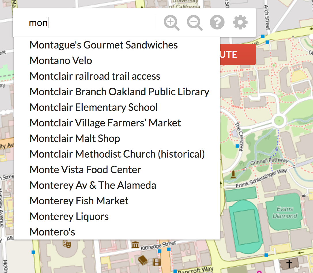
We would like to implement an Autocomplete system where a user types in a partial query string, like “Mont”, and is returned a list of locations that have “Mont” as a prefix. To do this, implement getLocationsByPrefix in AugmentedStreetMapGraph.java, where the prefix is the partial query string.

The prefix will be a cleaned name for search. That is:

• everything except characters A through Z and spaces removed, and
• everything is lowercased.

This method should return a list containing the full names of all locations whose cleaned names share the cleaned query string prefix, without duplicates.

Runtime

Assuming that the lengths of the names are bounded by some constant, querying for prefix of length s should take \(\Theta(k)\) time where k is the number of words sharing the prefix. As with Part III’s closest operation, you’ll need to add some sort of additional data structure as an instance variable to your AugmentedStreetMapGraph in order to support this operation efficiently.

Exercise: getLocations

The user should also be able to search for places of interest. Implement getLocations in AugmentedStreetMapGraph which collects a List of Maps containing information about the matching locations - that is, locations whose cleaned name match the cleaned query string exactly. This is not a unique list and should contain duplicates if multiple locations share the same name (i.e. Top Dog, Bongo Burger). See the Javadocs for the information each Map should contain.

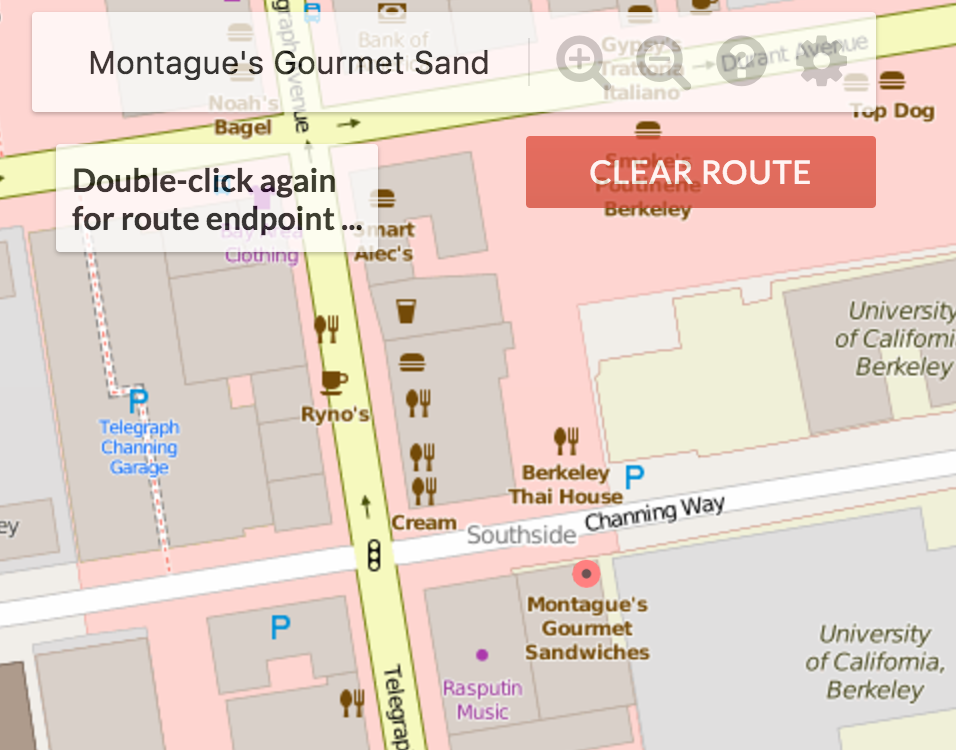
Implementing this method correctly will allow the web application to draw red dot markers on each of the matching locations. Note that because the location data is not very accurate, the markers may be a bit off from their real location. For example, the west side top dog is on the wrong side of the street!

Runtime

Suppose there are k results. Your query should run in \(\Theta(k)\) time.

V. Turn-by-turn Navigation (Optional)

To be explicitly clear, by completing this section you will not receive any additional points. This is only meant to be an additional challenge if you have time after finishing the first parts.

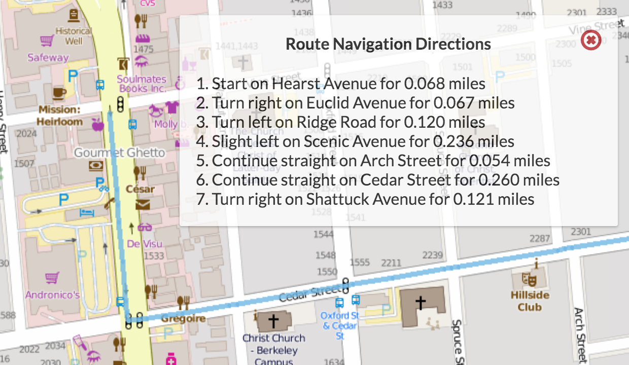
As an optional extra-challenging feature that is not for credit, you can use your A* search route to generate a sequence of navigation instructions that the server will then be able to display when you create a route. To do this, implement the additional method routeDirections in your Router class. This part of the project is not worth any points, but it is awfully cool.

To save effort, you’ll want to use various methods in the NavigationDirections class, for example bearing.

How we will represent these navigation directions will be with the NavigationDirection object defined within Router.java. A direction will follow the format of “DIRECTION on WAY for DISTANCE miles”. Note that DIRECTION is an int that will correspond to a defined String direction in the directions map, which has 8 possible options:

• “Start”
• “Continue straight”
• “Slight left/right”
• “Turn left/right”
• “Sharp left/right”

What direction a given NavigationDirection should have will be dependent on your previous node and your current node along the computed route. Specifically, the direction will depend on the relative bearing between the previous node and the current node, and should be as followed:

• Between -15 and 15 degrees the direction should be “Continue straight”.
• Beyond -15 and 15 degrees but between -30 and 30 degrees the direction should be “Slight left/right”.
• Beyond -30 and 30 degrees but between -100 and 100 degrees the direction should be “Turn left/right”.
• Beyond -100 and 100 degrees the direction should be “Sharp left/right”.

The navigation will be a bit complicated due to the fact that the previous and current node at a given point on your route may not necessarily represent a change in the “way” that you’re currently on, where a way is the name of a street or path that you’re currently traveling along. That is, if your route is from vertex 38623 to 2398471 to 1239871, these might all be the same street, and driving directions aren’t useful if they keep saying “Go straight on Shattuck. Go Straight on Shattuck. Go straight on Shattuck.” As a result, what you will need to do as you iterate through your route is keep track of when you actually change ways, and if so generate the correct distance for the NavigationDirection representing the way you were previously on, add it to the list, and continue. If you happen to change ways to one without a name, it’s way should be set to the constant “unknown road”.

As an example, suppose when calling routeDirections for a given route, the first node you remove is on the way “Shattuck Avenue”. You should create a NavigationDirection where the direction corresponds to “Start”, and as you iterate through the rest of the nodes, keep track of the distance along this way you travel. When you finally get to a node that is not on “Shattuck Avenue”, you should make sure NavigationDirection should have the correct total distance traveled along the previous way to get there (suppose this is 0.5 miles). As a result, the very first NavigationDirection in your returned list should represent the direction “Start on Shattuck Avenue for 0.5 miles.”. From there, your next NavigationDirection should have the name of the way your current node is on, the direction should be calculated via the relative bearing, and you should continue calculating its distance like the first one.

After you have implemented this properly you should be able to view your directions on the server by plotting a route and clicking on the button on the top right corner of the screen.

IV. Going Even Further (Optional)

You’re welcome to go even further. If you come up with something cool, let us know.

Heroku Deployment

Creation of a JAR with dependencies

A JAR with dependencies is a type of JAR that includes all your code from the external libraries (dependencies) used in the project. When we deploy an application on external server we need this kind of JAR which is self-sufficient(does not depend on anything else) and is enough to run the entire code.

An important step for this is to package all the resources, i.e, static data files (images, etc in our case) within this JAR itself.

1. Configuring JAR

• Go to File -> Project Structure -> Artifacts -> + -> JAR -> from modules with dependencies
• Your current module will be selected
• In the Main Class field click on the folder icon on the right end and select MapServer.java
• Next select the option extract to the target JAR

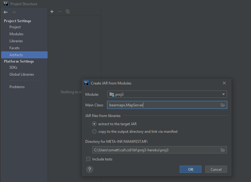
• The field Directory for META-INF/MANIFEST.MF should be populated. Ensure that the path given here is only up to the base (proj3) directory.
• Click OK which should take you back to the Artifacts window.
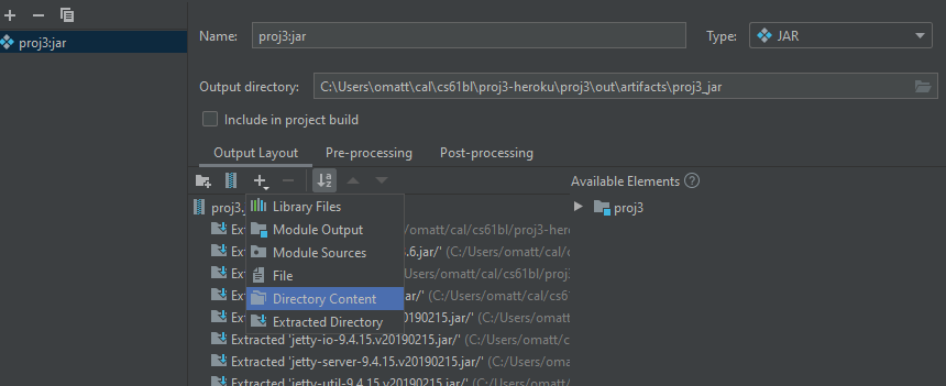
• In the Output Layout tab, click +, select Directory Content and select the library-su20 directory. This will place the contents of library-su20 into the jar

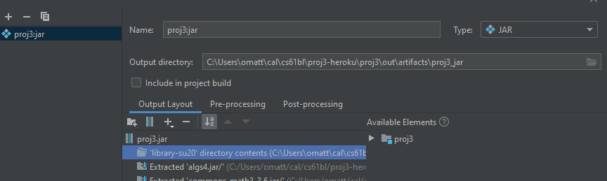
• Select Apply and Ok.

2. Configuring your code

2.1 Editing Paths

Since we have placed the data directory in the jar itself, we need to change the file paths of our images and other xml files. This should be as simple as updating the BASE_DIR_PATH from ../library-su20/ to ./.

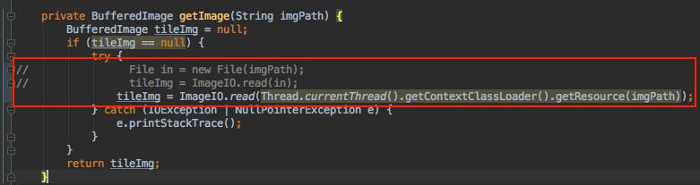
2.2 Reading files

Since the files are present in the JAR now, we need to change the way we read them in RasterAPIHandler and StreetMapGraph. To read files from jar we make use of Thread.currentThread().getContextClassLoader().getResource(filePath) and Thread.currentThread().getContextClassLoader().getResource(filePath) functions. These functions help us access content from our resources root.

• This is how the code for reading an image in RasterAPIHandler should look like

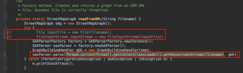
• This is how the code for reading an image in StreetMapGraph should look like

2.2 Configuring port

Since we are deploying our application on an external server we need to configure the port we want our application to run on.

• Add the following function to MapServerInitializer. This function returns the appropriate port to be used by the application. It sets the default to 4567.

  private static int getHerokuAssignedPort() {
        ProcessBuilder processBuilder = new ProcessBuilder();
        if (processBuilder.environment().get("PORT") != null) {
            return Integer.parseInt(processBuilder.environment().get("PORT"));
        }
        return 4567; //return default port if heroku-port isn't set (i.e. on localhost)
    }
  

• Call the above method in first line of the initializeServer function using port(getHerokuAssignedPort());
• This is how it looks like

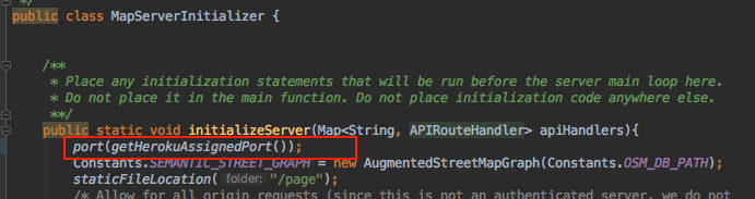
Building JAR

• Go to Build -> Build Artifacts...
• After this you will be able to see the JAR file created in your base project directory (proj3) under the path out/artifacts/<base-project-directory-name>_jar/<base-project-directory-name>.jar. This is JAR with dependencies.

Testing your JAR

On the terminal, navigate to the path where the JAR was created and run java -jar <jar-name>.jar. Your application should start running and work as it worked when you ran it from IntelliJ. Now we are ready to deploy this on Heroku!

Heroku Deployment

Onetime setup steps

1. Setup your free Heroku account here. If you already have an account you should be able to skip this step.
2. Install and setup Heroku Command Line Interface (CLI) by following the instructions here.
3. Make sure you have completed log-in steps to Heroku cli using the command heroku login
4. Run command heroku create bearmaps-<repo-id(For example, bearmaps-su20-s123) in the base project directory (proj3). This will create a Heroku app with the name bearmaps-<repo-id> and would be visible in your Dashboard at https://dashboard.heroku.com/apps
5. Install Heroku deploy plugin using heroku plugins:install heroku-cli-deploy

Deploying

• Deploy your JAR using the following Command heroku deploy:jar <path-to-JAR-file>.jar --app bearmaps-<repo-id> --jdk 11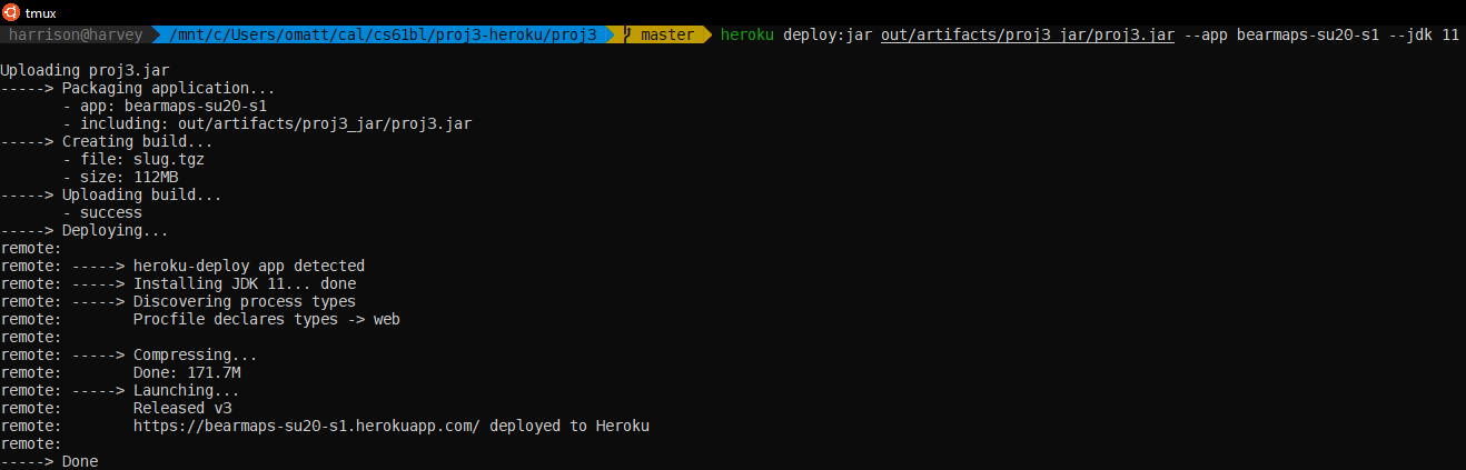
• Your App will be deployed at http://bearmaps-<repo-id>.herokuapp.com/map.html.

  Make sure that you are using http not https or you there will likely be an error.

• You can go to Heroku dashboard and explore different features. Click on More to see logs of your app.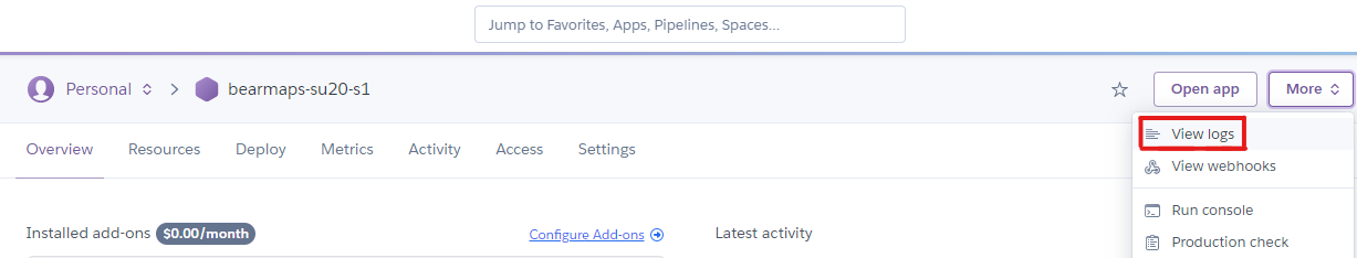

FAQ

Unable to read image and/or xml files.

Make sure that the paths are changed correctly and you have included the contents of library-sp19 folder in the jar output, while configuring artifact.>

FAQ

I provided the correct String[][] output but it doesn’t show up!

In order for something to show up on test.html, you need to set query_success to true, and in order for something to show up on map.html all the parameters must be set.

I checked every element of map I return with RasterAPIHandler.processRequest and they’re all correct, but still nothing is appearing.

If you’re using notation that you learned somewhere that looks like {{}} to initialize your map, you should not be doing so. Double-braces notation is an unintended “feature” of Java that is actually a terrible plan for a number of reasons.

My initial map doesn’t fill up the screen!

If your monitor resolution is high & the window is full screen, this can happen. Refer to the reference solution to see if yours looks similar.

Zooming out behaves weirdly

This is a known issue in the front end and is not your code’s fault. We’re hoping to fix this ASAP.

I don’t draw the entire query box on some inputs because I don’t intersect enough tiles.

That’s fine, that’ll happen when you go way to the edge of the map. For example, if you go too far west, you’ll never reach the bay because it does not exist.

I’m getting funky behavior with moving the map around, my image isn’t large enough at initial load, after the initial load, I can’t move the map, or after the initial load, I start getting NaN as input params.

These all have to do with your returned parameters being incorrect. Make sure you’re returning the exact parameters as given in the project 3 slides or the test .html files.

I’m failing the local router tests and I don’t know why. It says java.lang.AssertionError: The test says: Expected: [760706748, 3178363987, …], but Actual:[]

This is probably because you are including locations of places like Bongo Burger in your KDTree. As noted in the spec above, when handling a call to closest, you should only include vertices that have neighbors, otherwise closest may a return a node with no neighbors, which is trivially unable to act as a useful starting or ending node (since it literally cannot be reached).

I sometimes pass the timing tests when I submit, but not consistently.

If you have a efficient solution: it will always pass. We have yet to fail the timing test with or any of the other staff’s solutions over a lot of attempts to check for timing volatility.

If you have a borderline-efficient solution: it will sometimes pass. That’s just how it is, and there really isn’t any way around this if we want the autograder to run in a reasonable amount of time.

How do query boxes or bounding boxes make sense on a round world?

For the rastering part of the project, we assume the world is effectively flat on the scale of the map you’re looking at. In truth, each image doesn’t cover a rectangular area, but rather a “spherical cap”.

I’m missing xml files and/or library-su20 is not updated.

Go into the library-su20 directory and try the commands git submodule update --init followed by git checkout master.

My getLocations method works fine and I get markers on the map when I click on a search result but the Autograder test for getLocations method fails.

Try verifying that your getLocations method works for the cleaned strings as well other than the unclean strings

I pass all the local tests, but I’m getting a NoSuchElementException in the autograder

The autograder uses randomized sources and targets. Some targets may not be reachable from all sources. In these cases, you can do anything you want except let your program crash (e.g.return an empty list of longs).

Submission

The autograder will be released by the beginning of next week. In the meantime, you should use client side tests (test.html, map.html, the provided JUnit tests, etc.).

We have your git configured to avoid pushing all the extra stuff we don’t care about, e.g. html files DO NOT submit or upload to git any xml or png files. Attempting to do so will eat your internet bandwidth, cause the autograder to fail, and possibly even crash your computer.

Resources

Project 3 video playlist

Project 3 slides

FileDisplayDemo: FileDisplayDemo.html

Summer 2020 reference version: http://bearmaps-su20-s1.herokuapp.com/map.html

Course collaboration policy

Acknowledgements

Data made available by OSM under the Open Database License. This project also uses the JavaSpark web framework and Google Gson library.

Alan Yao for creating the original version of this project. Colby Yuan and Eli Lipsitz for substantial refactoring of the front end. Rahul Nangia for substantial refactoring of the back end.